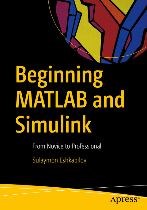
Beginning MATLAB and Simulink (eBook)
XXV, 524 Seiten
Apress (Verlag)
978-1-4842-5061-7 (ISBN)
- Get started using MATLAB and Simulink
- Carry out data visualization with MATLAB
- Gain the programming and modeling essentials of MATLAB
- Build a GUI with MATLAB
- Work with integration and numerical root finding methods
- Apply MATLAB to differential equations-based models and simulations
- Use MATLAB for data science projects
Employ essential and hands-on tools and functions of the MATLAB and Simulink packages, which are explained and demonstrated via interactive examples and case studies. This book contains dozens of simulation models and solved problems via m-files/scripts and Simulink models which help you to learn programming and modeling essentials. You'll become efficient with many of the built-in tools and functions of MATLAB/Simulink while solving engineering and scientific computing problems. Beginning MATLAB and Simulink explains various practical issues of programming and modelling in parallel by comparing MATLAB and Simulink. After reading and using this book, you'll be proficient at using MATLAB and applying the source code from the book's examples as templates for your own projects in data science or engineering. What You Will LearnGet started using MATLAB and SimulinkCarry out data visualization with MATLABGain the programming and modeling essentials of MATLABBuild a GUI with MATLABWork with integration and numerical root finding methodsApply MATLAB to differential equations-based models and simulationsUse MATLAB for data science projectsWho This Book Is ForEngineers, programmers, data scientists, and students majoring in engineering and scientific computing.
Table of Contents 5
About the Author 17
About the Technical Reviewers 18
Acknowledgments 20
Introduction 21
Chapter 1: Introduction to MATLAB 24
MATLAB’s Menu Panel and Help 24
The MATLAB Environment 30
Working in the Command Window 32
Command Window and Variables 34
Using Variables 34
When to Use the Command Window 41
Different Variables and Data Sets in MATLAB 46
Numerical Data/Arrays 48
NaN (Not-a-Number) 56
Character Types of Variables 61
Function Handle 63
Logical Arrays 67
Table Arrays 71
Cell Arrays 73
Structure Arrays 77
Complex Numbers 82
Precision 82
M-File and MLX–File Editors 83
M-File Editor 83
MLX-File Editor 85
% Comments 88
Closing the MATLAB Window 95
Summary 95
References 95
Exercises for Self-Testing 96
Exercise 1 96
Exercise 2 96
Exercise 3 96
Exercise 4 97
Exercise 5 97
Exercise 6 97
Exercise 7 97
Exercise 8 97
Exercise 9 97
Exercise 10 98
Exercise 11 98
Exercise 12 98
Exercise 13 99
Exercise 14 99
Exercise 15 99
Exercise 16 100
Exercise 17 100
Exercise 18 100
Exercise 19 100
Exercise 20 100
Exercise 21 101
Exercise 22 101
Exercise 23 101
Exercise 24 102
Exercise 25 102
Exercise 26 103
Exercise 27 103
Exercise 28 103
Exercise 29 103
Exercise 30 103
Exercise 31 104
Exercise 32 105
Exercise 33 105
Exercise 34 106
Exercise 35 106
Exercise 36 106
Exercise 37 107
Exercise 38 107
Exercise 39 107
Exercise 40 108
Exercise 41 109
Exercise 42 110
Exercise 43 112
Exercise 44 112
Chapter 2: Programming Essentials 113
Writing M/MLX-Files 113
How to Create an M/MLX-File 116
Warnings in Scripts 116
Errors in Scripts 120
Example 1 120
Example 2 123
Example 3 125
Example 4 127
Example 5 130
Cell Mode 135
Debugging Mode 139
M-Lint Code Check 140
Code Profiling 140
Dependency Report 141
P-Codes 141
Some Remarks About Scripts/M/MLX-Files 143
Display and Printout Operators: display, sprintf, and fprintf 143
Example 1 144
Example 2 145
fprintf() 146
The if, else, elseif, end and switch, case, end Control Statements 152
Example 1 154
Example 2 155
Example 3 157
Case 1 160
Case 2 161
Case 3 161
Example 4 162
Loop Control Statements: while, for, continue, break, and end 163
Example 1 164
Example 2 165
Example 3 169
Example 4 172
Example 5 173
Example 6 176
Example 7 179
Example 8 180
Memory Allocation 181
Example 9 182
Example 10 184
Example 11 185
Example 12 187
Example 13 189
Example 14 194
Example 15 197
Example 16 198
Symbol References in Programming 200
Asterisk 201
At (@) Sign 201
Colon 202
Comma 202
Curly Brackets 202
Dollar Sign 203
Dot 203
Dot-Dot 203
Dot-Dot-Dot (Ellipsis) 203
Parentheses 204
Percent 204
Semicolon 205
Single Quotes 206
Slash and Backslash 206
Square Brackets 206
Function Files 207
Example 1 209
Example 2 211
Example 3 212
Example 4 213
Most Common Errors with Function Files 216
Varying Number of Inputs and Outputs 218
Example 5 219
Example 6 221
Example 7 224
Task 1 224
Task 2 225
Nested and Sub-Functions of Function Files 234
Example 8 235
Function Files Within M-Files 237
Example 9 237
Summary of Scripts and Function Files 239
Inline Functions 240
Example 1 240
Example 2 241
Example 3 241
Anonymous Functions with Handles (@) 242
Example 1 242
Example 2 243
Example 3 243
How to Improve Script Performance 244
Chapter 3: Graphical User Interface Model Development 245
GUIDE 245
Example 1: Building a 2D Plot 250
Example 2: Adding Functionality 257
Example 3: Solving a Quadratic Equation 260
Building the GUI 260
Editing the Callback Functions 263
GUI Dialogs and Message Boxes 268
Error Dialog 269
Warning Message 269
F1 Help/Message Box 269
General Syntax 271
Input Dialog 272
Question Dialog 272
Making a Choice 273
Providing Input to an Equation 277
Chapter 4: MEX Files, C/C++, and Standalone Applications 280
Verifying Compilers 281
Generating C Code 281
Creating MEX Files from Other Languages 288
Building Standalone Applications 289
Chapter 5: Simulink Modeling Essentials 295
Simulink Modeling 295
Example: Arithmetic Calculations 297
Example: Modeling Simple Arithmetic Operations 301
Performing Matrix Operations 305
Computing Values of Functions 310
Input/Output Signals from/to the MATLAB Workspace 317
Simulating a Mechanical System 320
Working with a Second Order Differential Equation 328
Simulink Model Analysis and Diagnostics 333
Code Generation 334
Model Advisor 335
Summary 341
Exercises for Self-Testing 341
Exercise 1 341
Exercise 2 341
Exercise 3 342
Exercise 4 342
Exercise 5 343
Exercise 6 344
Exercise 7 344
Exercise 8 345
Exercise 9 346
Exercise 10 347
Exercise 11 348
Exercise 12 349
Exercise 13 350
Exercise 14 351
Exercise 15 351
Exercise 16 352
Exercise 17 352
Exercise 18 353
Exercise 19 353
Exercise 20 354
Exercise 21 354
Exercise 22 355
Exercise 23 355
Exercise 24 356
Exercise 25 357
Exercise 26 357
Exercise 27 358
Exercise 28 358
Exercise 29 359
Exercise 30 360
Exercise 31 361
Exercise 32 361
Exercise 33 362
Exercise 34 362
Exercise 35 362
Chapter 6: Plots and Data Visualization 363
Basics of Plot Building 363
PLOT() 364
Example 1: Plotting Two Rows of Data 364
Example 2: Plotting Function Values 365
Example 3: Building a Histogram 367
TITLE, XLABEL, YLABEL, AXIS, GRID, and LEGEND 368
TITLE() 368
XLABEL, YLABEL, and ZLABEL 368
AXIS 368
GRID 369
Example 4: Plotting a Unit Circle with Plot Tools 369
LINE and MARKER Specifiers 370
Example 5: Plotting Sine Function Values with Plot Tools 373
Special Characters 374
Example 6: Plotting Sine Function Values with Plot Tools 375
Plot Two Data Sets in Two Y–Y Axes 376
Example 7: Plotting Two Function Values on Y-Y Axes 376
Sub-plots 379
Example 8: Building Sub-Plots of Functions 379
LEGEND 381
HOLD 381
Example 9: Plotting a Few Function Values in One Plot 381
Example 10: Plotting Function Values with Different Line Markers and Colors 382
EZPLOT, FPLOT, and FIMPLICIT with Function Handles (@) 384
Example 11: Plotting a Mathematical Expression with ezplot() 384
GTEXT, TEXT, and GINPUT 385
Example 12: Locate and Display Minimum Values of a Function Plot in a Plot Figure 386
Axis Ticks and Tick Labels 388
Example 13: Display X-Axis Tick Labels 389
Figure Handles 390
Example 14: Working with Figure Handles 390
3D Surface Plots 392
Example 15: Creating a 3D Pie Plot with pie() 392
Example 16: Creating a 3D Surface Plot with ezsurf() 393
Example 17: Creating a 3D Mesh Plot with ezmesh() 394
Example 18: Creating a 3D Surface-Contour Plot with ezsurfc() 394
Example 19: Creating a 3D Plot of an Electric Potential Field 395
Example 20: Creating 3D Plots with waterfall() and ribbon() 398
3D Line Plots and Animations 400
Example 21: Building 3D Line Plots and Animated 3D Line Plots with plot3(), comet3(), and ezplot3() 400
Animated Plots 402
Example 22: Building an Animated Plot with getframe() 402
Example 23: Building an Animated Plot with drawnow 403
Example 24: Building an Animated Plot with drawnow 403
Example 25: Building an Animated Plot of a Projectile with getframe() 404
Summary 405
Exercises for Self-Testing 406
Exercise 1 406
Exercise 2 407
Exercise 3 407
Exercise 4 407
Exercise 5 408
Exercise 6 409
Exercise 7 409
Exercise 8 409
Exercise 9 410
Exercise 10 410
Exercise 11 410
Exercise 12 411
Exercise 13 411
Exercise 14 411
Exercise 15 411
Exercise 16 412
Exercise 17 412
Exercise 18 413
Exercise 19 413
Exercise 20 414
Exercise 21 414
Exercise 22 414
Exercise 23 415
Exercise 24 415
Exercise 25 416
Chapter 7: Linear Algebra 417
Introduction to Linear Algebra 417
Matrix Properties and Operators 419
Simulink Blocks for Matrix Determinant, Diagonal Extraction, and Transpose 420
Matrix Inverse or Inverse Matrix 424
Simulink Blocks for Inverse Matrix 425
Example 1: Solving a System of Linear Equations 428
Simulink Modeling 434
Example 2: Embedding a MATLAB Function Block to Compute the Determinant and Solve Linear Equations 437
Example 3: Accuracy of Solver Functions of Linear Equations 439
Example 4: Efficiency of Solver Functions of Linear Equations 442
Example 5: Solving Linear Equations ([A]{x} = [b]) by Changing Values of [b] 445
Matrix Operations 448
Example: Performing Matrix Operations 451
Standard Matrix Generators 460
Vector Spaces 465
Polynomials Represented by Vectors 467
Simulink Model Based Solution of Polynomials 469
Eigen-Values and Eigen-Vectors 471
Matrix Decomposition 474
QR Decomposition 474
Example: Computing QR Decomposition of a 5-by-5 Matrix 475
LU Decomposition 477
Example: Computing LU Composition of a 3-by-3 Pascal Matrix 478
Cholesky Decomposition 480
Schur Decomposition 484
Singular Value Decomposition (SVD) 487
Logic Operators, Indexes, and Conversions 489
Logical Indexing 490
Example: Logical Indexing to locate and Substitute Elements of A Matrix 493
Conversions 495
Example: Creating Character Strings with char() 498
Summary 500
References 501
Exercises for Self-Testing 502
Exercise 1 502
Exercise 2 503
Exercise 3 503
Exercise 4 504
Exercise 5 504
Exercise 6 505
Exercise 7 505
Exercise 8 505
Exercise 9 506
Exercise 10 506
Exercise 11 506
Exercise 12 507
Exercise 13 507
Exercise 14 507
Exercise 15 507
Exercise 16 508
Exercise 17 508
Exercise 18 508
Exercise 19 508
Exercise 20 509
Exercise 21 509
Exercise 22 509
Exercise 23 509
Exercise 24 509
Exercise 25 510
Chapter 8: Ordinary Differential Equations 511
Classifying ODEs 512
Example 1: Unconstrained Growth of Biological Organisms 513
Example 2: Radioactive Decay 513
Example 3: Newton’s Second Law 514
Analytical Methods 515
DSOLVE 516
Example 1: Using dsolve 516
Example 2: Plotting from dsolve 516
Example 3: Adding an Unspecified Parameter 518
Second-Order ODEs and a System of ODEs 519
Example 1: dsolve with a Second-Order ODE 519
Example 2: System ODEs 520
Example 3: Unsolvable Solutions Using dsolve 521
Example 4: Computing an Analytical Solution 522
Example 5: An Interesting ODE 522
Example 6: Responding to No Analytical Solution 523
Laplace Transforms 524
Example 1: First Laplace Transform 525
LAPLACE/ILAPLACE 526
Example 2: Using LAPLACE 527
Example 3: A Final LAPLACE 527
Example 4: Comparing LAPLACE/ILAPLACE with DSOLVE 528
Example 5: Convergent Answers 530
Example 6: No Analytical Solution 532
Example 7: Demonstrating Efficiency and Effortlessness 533
References 536
Index 537
| Erscheint lt. Verlag | 28.11.2019 |
|---|---|
| Zusatzinfo | XXV, 524 p. 374 illus., 364 illus. in color. |
| Sprache | englisch |
| Themenwelt | Mathematik / Informatik ► Informatik ► Programmiersprachen / -werkzeuge |
| Informatik ► Theorie / Studium ► Compilerbau | |
| Mathematik / Informatik ► Mathematik ► Angewandte Mathematik | |
| Mathematik / Informatik ► Mathematik ► Computerprogramme / Computeralgebra | |
| Naturwissenschaften | |
| Schlagworte | Code • Development • engineer • Functions • Math • MATLAB • programming • SIMULINK • Software • Tutorial |
| ISBN-10 | 1-4842-5061-3 / 1484250613 |
| ISBN-13 | 978-1-4842-5061-7 / 9781484250617 |
| Haben Sie eine Frage zum Produkt? |
Größe: 25,7 MB
DRM: Digitales Wasserzeichen
Dieses eBook enthält ein digitales Wasserzeichen und ist damit für Sie personalisiert. Bei einer missbräuchlichen Weitergabe des eBooks an Dritte ist eine Rückverfolgung an die Quelle möglich.
Dateiformat: PDF (Portable Document Format)
Mit einem festen Seitenlayout eignet sich die PDF besonders für Fachbücher mit Spalten, Tabellen und Abbildungen. Eine PDF kann auf fast allen Geräten angezeigt werden, ist aber für kleine Displays (Smartphone, eReader) nur eingeschränkt geeignet.
Systemvoraussetzungen:
PC/Mac: Mit einem PC oder Mac können Sie dieses eBook lesen. Sie benötigen dafür einen PDF-Viewer - z.B. den Adobe Reader oder Adobe Digital Editions.
eReader: Dieses eBook kann mit (fast) allen eBook-Readern gelesen werden. Mit dem amazon-Kindle ist es aber nicht kompatibel.
Smartphone/Tablet: Egal ob Apple oder Android, dieses eBook können Sie lesen. Sie benötigen dafür einen PDF-Viewer - z.B. die kostenlose Adobe Digital Editions-App.
Zusätzliches Feature: Online Lesen
Dieses eBook können Sie zusätzlich zum Download auch online im Webbrowser lesen.
Buying eBooks from abroad
For tax law reasons we can sell eBooks just within Germany and Switzerland. Regrettably we cannot fulfill eBook-orders from other countries.
aus dem Bereich


