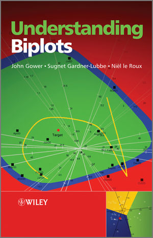
Understanding Biplots
John Wiley & Sons Inc (Verlag)
978-0-470-01255-0 (ISBN)
- Titel ist leider vergriffen;
keine Neuauflage - Artikel merken
Biplots are a graphical method for simultaneously displaying two kinds of information; typically, the variables and sample units described by a multivariate data matrix or the items labelling the rows and columns of a two-way table. This book aims to popularize what is now seen to be a useful and reliable method for the visualization of multidimensional data associated with, for example, principal component analysis, canonical variate analysis, multidimensional scaling, multiplicative interaction and various types of correspondence analysis. Understanding Biplots:
• Introduces theory and techniques which can be applied to problems from a variety of areas, including ecology, biostatistics, finance, demography and other social sciences.
• Provides novel techniques for the visualization of multidimensional data and includes data mining techniques.
• Uses applications from many fields including finance, biostatistics, ecology, demography.
• Looks at dealing with large data sets as well as smaller ones.
• Includes colour images, illustrating the graphical capabilities of the methods.
• Is supported by a Website featuring R code and datasets.
Researchers, practitioners and postgraduate students of statistics and the applied sciences will find this book a useful introduction to the possibilities of presenting data in informative ways.
John C. Gower, Department of Mathematics, The Open University, Milton Keynes, UK. Over 100 papers. Books include Gower & Hand (1996) Biplots, in which the authors developed a unified theory of biplots. Sugnet Gardner, British American Tobacco, Stellenbosch, South Africa. Niel J. le Roux, Department of Statistics and Actuarial Science, University of Stellenbosch , South Africa.
Preface xi
1 Introduction 1
1.1 Types of biplots 2
1.2 Overview of the book 5
1.3 Software 7
1.4 Notation 7
1.4.1 Acronyms 9
2 Biplot basics 11
2.1 A simple example revisited 11
2.2 The biplot as a multidimensional scatterplot 14
2.3 Calibrated biplot axes 20
2.3.1 Lambda scaling 24
2.4 Refining the biplot display 32
2.5 Scaling the data 36
2.6 A closer look at biplot axes 37
2.7 Adding new variables: the regression method 44
2.8 Biplots and large data sets 47
2.9 Enclosing a configuration of sample points 50
2.9.1 Spanning ellipse 53
2.9.2 Concentration ellipse 54
2.9.3 Convex hull 57
2.9.4 Bagplot 58
2.9.5 Bivariate density plots 62
2.10 Buying by mail order catalogue data set revisited 64
2.11 Summary 66
3 Principal component analysis biplots 67
3.1 An example: risk management 67
3.2 Understanding PCA and constructing its biplot 71
3.2.1 Representation of sample points 72
3.2.2 Interpolation biplot axes 74
3.2.3 Prediction biplot axes 77
3.3 Measures of fit for PCA biplots 80
3.4 Predictivities of newly interpolated samples 94
3.5 Adding new axes to a PCA biplot and defining their predictivities 98
3.6 Scaling the data in a PCA biplot 103
3.7 Functions for constructing a PCA biplot 107
3.7.1 Function PCAbipl 107
3.7.2 Function PCAbipl.zoom 115
3.7.3 Function PCAbipl.density 115
3.7.4 Function PCAbipl.density.zoom 116
3.7.5 Function PCA.predictivities 117
3.7.6 Function PCA.predictions.mat 117
3.7.7 Function vector.sum.interp 117
3.7.8 Function circle.projection.interactive 118
3.7.9 Utility functions 118
3.8 Some novel applications and enhancements of PCA biplots 119
3.8.1 Risk management example revisited 119
3.8.2 Quality as a multidimensional process 123
3.8.3 Using axis predictivities in biplots 128
3.8.4 One-dimensional PCA biplots 128
3.8.5 Three-dimensional PCA biplots 135
3.8.6 Changing the scaffolding axes in conventional two-dimensional PCA biplots 138
3.8.7 Alpha-bags, kappa-ellipses, density surfaces and zooming 139
3.8.8 Predictions by circle projection 139
3.9 Conclusion 144
4 Canonical variate analysis biplots 145
4.1 An example: revisiting the Ocotea data 145
4.2 Understanding CVA and constructing its biplot 153
4.3 Geometric interpretation of the transformation to the canonical space 157
4.4 CVA biplot axes 160
4.4.1 Biplot axes for interpolation 160
4.4.2 Biplot axes for prediction 160
4.5 Adding new points and variables to a CVA biplot 162
4.5.1 Adding new sample points 162
4.5.2 Adding new variables 162
4.6 Measures of fit for CVA biplots 163
4.6.1 Predictivities of new samples and variables 168
4.7 Functions for constructing a CVA biplot 169
4.7.1 Function CVAbipl 169
4.7.2 Function CVAbipl.zoom 170
4.7.3 Function CVAbipl.density 170
4.7.4 Function CVAbipl.density.zoom 170
4.7.5 Function CVAbipl.pred.regions 170
4.7.6 Function CVA.predictivities 171
4.7.7 Function CVA.predictions.mat 172
4.8 Continuing the Ocotea example 172
4.9 CVA biplots for two classes 178
4.9.1 An example of two-class CVA biplots 178
4.10 A five-class CVA biplot example 185
4.11 Overlap in two-dimensional biplots 189
4.11.1 Describing the structure of overlap 189
4.11.2 Quantifying overlap 191
5 Multidimensional scaling and nonlinear biplots 205
5.1 Introduction 205
5.2 The regression method 206
5.3 Nonlinear biplots 208
5.4 Providing nonlinear biplot axes for variables 212
5.4.1 Interpolation biplot axes 215
5.4.2 Prediction biplot axes 218
5.4.2.1 Normal projection 220
5.4.2.2 Circular projection 222
5.4.2.3 Back-projection 226
5.5 A PCA biplot as a nonlinear biplot 227
5.6 Constructing nonlinear biplots 229
5.6.1 Function Nonlinbipl 230
5.6.2 Function CircularNonLinear.predictions 233
5.7 Examples 234
5.7.1 A PCA biplot as a nonlinear biplot 234
5.7.2 Nonlinear interpolative biplot 236
5.7.3 Interpolating a new point into a nonlinear biplot 237
5.7.4 Nonlinear predictive biplot with Clark’s distance 237
5.7.5 Nonlinear predictive biplot with square root of Manhattan distance 242
5.8 Analysis of distance 243
5.8.1 Proof of centroid property for interpolated points in AoD 249
5.8.2 A simple example of analysis of distance 250
5.9 Functions AODplot and PermutationAnova 253
5.9.1 Function AODplot 253
5.9.2 Function PermutationAnova 254
6 Two-way tables: biadditive biplots 255
6.1 Introduction 255
6.2 A biadditive model 256
6.3 Statistical analysis of the biadditive model 256
6.4 Biplots associated with biadditive models 260
6.5 Interpolating new rows or columns 261
6.6 Functions for constructing biadditive biplots 262
6.6.1 Function biadbipl 262
6.6.2 Function biad.predictivities 265
6.6.3 Function biad.ss 267
6.7 Examples of biadditive biplots: the wheat data 267
6.8 Diagnostic biplots 283
7 Two-way tables: biplots associated with correspondence analysis 289
7.1 Introduction 289
7.2 The correspondence analysis biplot 290
7.2.1 Approximation to Pearson’s chi-squared 290
7.2.2 Approximating the deviations from independence 291
7.2.3 Approximation to the contingency ratio 292
7.2.4 Approximation to chi-squared distance 293
7.2.5 Canonical correlation approximation 296
7.2.6 Approximating the row profiles 298
7.2.7 Analysis of variance and generalities 299
7.3 Interpolation of new (supplementary) points in CA biplots 302
7.4 Other CA related methods 303
7.5 Functions for constructing CA biplots 306
7.5.1 Function cabipl 306
7.5.2 Function ca.predictivities 310
7.5.3 Function ca.predictions.mat 310
7.5.4 Functions indicatormat, construct.df,Chisq.dist 311
7.5.5 Function cabipl.doubling 312
7.6 Examples 312
7.6.1 The RSA crime data set 312
7.6.2 Ordinary PCA biplot of the weighted deviations matrix 345
7.6.3 Doubling in a CA biplot 346
7.7 Conclusion 354
8 Multiple correspondence analysis 365
8.1 Introduction 365
8.2 Multiple correspondence analysis of the indicator matrix 366
8.3 The Burt matrix 372
8.4 Similarity matrices and the extended matching coefficient 376
8.5 Category-level points 377
8.6 Homogeneity analysis 378
8.7 Correlational approach 381
8.8 Categorical (nonlinear) principal component analysis 383
8.9 Functions for constructing MCA related biplots 386
8.9.1 Function cabipl 386
8.9.2 Function MCAbipl 386
8.9.3 Function CATPCAbipl 391
8.9.4 Function CATPCAbipl.predregions 394
8.9.5 Function PCAbipl.cat 394
8.10 Revisiting the remuneration data: examples of MCA and categorical PCA biplots 394
9 Generalized biplots 405
9.1 Introduction 405
9.2 Calculating inter-sample distances 406
9.3 Constructing a generalized biplot 408
9.4 Reference system 408
9.5 The basic points 412
9.6 Interpolation 413
9.7 Prediction 415
9.8 An example 417
9.9 Function for constructing generalized biplots 420
10 Monoplots 423
10.1 Multidimensional scaling 423
10.2 Monoplots related to the covariance matrix 427
10.2.1 Covariance plots 427
10.2.2 Correlation monoplot 431
10.2.3 Coefficient of variation monoplots 431
10.2.4 Other representations of correlations 433
10.3 Skew-symmetry 436
10.4 Area biplots 440
10.5 Functions for constructing monoplots 441
10.5.1 Function MonoPlot.cov 441
10.5.2 Function MonoPlot.cor 442
10.5.3 Function MonoPlot.cor2 443
10.5.4 Function MonoPlot.coefvar 443
10.5.5 Function MonoPlot.skew 443
References 445
Index 449
| Erscheint lt. Verlag | 1.3.2011 |
|---|---|
| Verlagsort | New York |
| Sprache | englisch |
| Maße | 175 x 252 mm |
| Gewicht | 1152 g |
| Themenwelt | Mathematik / Informatik ► Mathematik ► Statistik |
| Mathematik / Informatik ► Mathematik ► Wahrscheinlichkeit / Kombinatorik | |
| ISBN-10 | 0-470-01255-2 / 0470012552 |
| ISBN-13 | 978-0-470-01255-0 / 9780470012550 |
| Zustand | Neuware |
| Haben Sie eine Frage zum Produkt? |
aus dem Bereich


