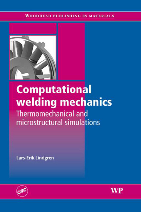
Computational welding mechanics (CWM) provides an important technique for modelling welding processes. Welding simulations are a key tool in improving the design and control of welding processes and the performance of welded components or structures. CWM can be used to model phenomena such as heat generation, thermal stresses and large plastic deformations of components or structures. It also has a wider application in modelling thermomechanical and microstructural phenomena in metals. This important book reviews the principles, methods and applications of CWM.The book begins by discussing the physics of welding before going on to review modelling methods and options as well as validation techniques. It also reviews applications in areas such as fatigue, buckling and deformation, improved service life of components and process optimisation. Some of the numerical methods described in the book are illustrated using software available from the author which allows readers to explore CWM in more depth.Computational welding mechanics is a standard work for welding engineers and all those researching welding processes and wider thermomechanical and microstructural phenomena in metals. - Highlights the principles, methods and applications of CWM- Discusses the physics of welding- Assesses modelling methods and validation techniques
Couplings and reference frames
As illustrated in the previous chapter, welding is a multi-physics problem where the physical phenomena are described by different coupled field equations that overlap or have a common boundary. Fortunately, many welding processes can be represented by simplified models. The main stream in CWM is the use of weakly coupled models where the physics in the weld is replaced by a heat input model. A general description about procedures for solving coupled systems is given in this chapter with focus on the use of the so-called staggered approach common in CWM, where the solution of the problem is split into a thermal and a mechanical phase. There are several options available in the thermal and mechanical analyses. One common concern is the choice of coordinate system. Most models use a fixed coordinate system. However, the moving heat source with near stationary conditions can be favourably treated by a moving coordinate system in some cases. This is described at the end of this chapter with references to papers in CWM using the Eulerian, moving, coordinate system. The next two chapters about finite element formulation for solution of the thermal and mechanical fields focus on the use of a fixed coordinate system.
3.1 Coupled systems and solution procedures
A large number of coupled systems exist and they are coupled in different ways [20]. There is the coupling between different components of a system with a common interface through which they interact, e.g. a fluid and solid boundary. Another type of coupling is the coupling between different physical phenomena in the same material, e.g. the coupling between temperature and deformation in the solid material.
Monolithic or partitioned treatment of the coupled systems is possible. The solution is advanced simultaneously in time in a monolithic treatment, whereas the field models are solved and advanced separately in time in a partitioned simulation. The latter is more common, has implementation advantages and can also be computationally more efficient. An example of partitioned analysis of a coupled system, taken from the papers by Felippa et al. [20, 21], is the two-field problem
x˙+4x−y=fty˙+6y−2x=gt
[3.1]
which, when discretised in time using a backward Euler algorithm, gives
+4h−h−2h1+6hn+1xn+1y=hn+1f+3nxhn+1g+ny
[3.2]
where h is the length of the time step and the left superscript is a time step counter. The initial conditions give the starting values needed for the algorithm. The solution of Eq. [3.2] is a monolithic treatment of the problem.
The basic idea for a staggered solution procedure is shown in Fig. 3.1. The solution is advanced in two separate steps, denoted Ax and Ay in the figure. A predictor, denoted P, is used when advancing the first field, x in this case. This is then substituted into the solution of the second field. This substitution is trivial and denoted S in the figure. The graph for the solution procedure (right part in Fig. 3.1) illustrates the logic and is usually drawn without the dashed lines. The approach can then be drawn as in Fig. 3.2, which explains why it is called a staggered approach. The staggered approach can be combined with a full step correction as illustrated in Fig. 3.3 to compute an improved predictor value Py, and the solution according to Fig. 3.1 is repeated once again. Box 3.1 compares the fully coupled solution and the staggered approach for solving Eq. [3.2].
Box 3.1
Demonstration of solution procedures for coupled systems in Eq. [3.1]
MapleTM is used to get the analytic solution of the coupled system of equations in Eq. [3.1], using the initial conditions x(0) = y(0) = 0 and f (t) = sin(t), g ≡ 0. The solution is
xt=184516r3r1e-1/3r¯2t+16r¯3r¯1e-1/3r2t-113cost+136sintyt=1845r1e-1/3r¯2t+r¯1e-1/3r2t-44cost+38sint
where the roots are
1=22+371155,r¯1=22−371155,r2=11+55,r¯2=11−55,r3=7+55,r¯3=7−55
The analytic solution is compared with the fully coupled solution of Eq. [3.2] and the solution using the staggered approach shown in Fig. 3.1. The difference between the two methods is quite small even when taking large time steps. The circles lie almost on the dashed lines. This can be seen in Fig. 3.4 where it can also be noted then that they both deviate considerably from the exact solution. Thus the requirement for accuracy is more important in this particular case. An accurate solution will require smaller time steps and then the staggered approach will be more efficient than the fully coupled approach.
Other improvements of the staggered approach include the use of augmentation methods [20, 21] where the equations for advancing the solution of one field are reformulated with information from the other field. This is illustrated in Section 3.2 where an augmentation method for thermoelasticity in [20] is related to the operator split approach in [22, 23].
3.2 Linearised coupled thermoelasticity
The different solution procedures for fully coupled thermomechanical problems are illustrated by an example taken from Armero and Simo [23]. The finite element formulas below are general, although the particular case is a one-dimensional problem.
3.2.1 One-dimensional thermoelasticity
The equation of motion for a uniaxial stress case without body forces is
σdx=ρu¨
[3.3]
where σ is the stress, u the displacement, ü the acceleration and ρ the density. The material behaviour for the linear thermoelastic material is taken as
=Eϵ−αT
[3.4]
where E is Young’s modulus and α is the coefficient of thermal expansion. It is assumed that the body is stress free at T = 0. Thus the temperature can be considered as the increase in temperature from the stress free state. Furthermore, we assume small strains, ,
=dudx
[3.5]
The three equations above can be used to derive the one-dimensional Navier’s equation, the equilibrium equation expressed in terms of the displacements,
d2udx2−EαdTdx=ρu¨
[3.6]
where the second term on the left hand side can now be interpreted as a volumetric load due to the thermal strains.
The energy balance in one-dimensional heat conduction can be written as
dqdx=ρcvT˙+EαTϵ˙
[3.7]
where q is the heat flux and cv is the heat capacity at constant volume. There is some variation in the use of the latter. Some references, for example [24, 25], use cp, which is the heat capacity at constant pressure. Others [26–29] use cv. This variation in notation was noticed by Carslaw and Jaeger [30]. The difference between these two quantities is negligible for solids and liquids. The notation c is used in the following. The equation includes mechanically generated heat [25, 27, 28].
Fourier’s law for heat flow gives
=−λg
[3.8]
where λ is the heat conductivity, and the temperature gradient, g, is computed as
=dTdx
[3.9]
These three equations give Duhamel’s heat conduction equation
T˙+EαTaϵ˙=λ∂2T∂x2
[3.10]
where Ta is the absolute temperature in K. The temperature T is the temperature difference with respect to the stress-free state according to Eq. [3.4], which can be given in different units, for example °F or °C. The equation is linearised to
T˙+EαTrefϵ˙=λ∂2T∂x2
[3.11]
where the left hand side is equal to the entropy change. The equation is linearised by assuming...
| Erscheint lt. Verlag | 23.1.2014 |
|---|---|
| Sprache | englisch |
| Themenwelt | Informatik ► Grafik / Design ► Digitale Bildverarbeitung |
| Mathematik / Informatik ► Informatik ► Theorie / Studium | |
| Technik ► Maschinenbau | |
| Wirtschaft | |
| ISBN-10 | 1-84569-355-8 / 1845693558 |
| ISBN-13 | 978-1-84569-355-8 / 9781845693558 |
| Haben Sie eine Frage zum Produkt? |
Größe: 10,6 MB
Kopierschutz: Adobe-DRM
Adobe-DRM ist ein Kopierschutz, der das eBook vor Mißbrauch schützen soll. Dabei wird das eBook bereits beim Download auf Ihre persönliche Adobe-ID autorisiert. Lesen können Sie das eBook dann nur auf den Geräten, welche ebenfalls auf Ihre Adobe-ID registriert sind.
Details zum Adobe-DRM
Dateiformat: PDF (Portable Document Format)
Mit einem festen Seitenlayout eignet sich die PDF besonders für Fachbücher mit Spalten, Tabellen und Abbildungen. Eine PDF kann auf fast allen Geräten angezeigt werden, ist aber für kleine Displays (Smartphone, eReader) nur eingeschränkt geeignet.
Systemvoraussetzungen:
PC/Mac: Mit einem PC oder Mac können Sie dieses eBook lesen. Sie benötigen eine
eReader: Dieses eBook kann mit (fast) allen eBook-Readern gelesen werden. Mit dem amazon-Kindle ist es aber nicht kompatibel.
Smartphone/Tablet: Egal ob Apple oder Android, dieses eBook können Sie lesen. Sie benötigen eine
Geräteliste und zusätzliche Hinweise
Buying eBooks from abroad
For tax law reasons we can sell eBooks just within Germany and Switzerland. Regrettably we cannot fulfill eBook-orders from other countries.
Größe: 7,5 MB
Kopierschutz: Adobe-DRM
Adobe-DRM ist ein Kopierschutz, der das eBook vor Mißbrauch schützen soll. Dabei wird das eBook bereits beim Download auf Ihre persönliche Adobe-ID autorisiert. Lesen können Sie das eBook dann nur auf den Geräten, welche ebenfalls auf Ihre Adobe-ID registriert sind.
Details zum Adobe-DRM
Dateiformat: EPUB (Electronic Publication)
EPUB ist ein offener Standard für eBooks und eignet sich besonders zur Darstellung von Belletristik und Sachbüchern. Der Fließtext wird dynamisch an die Display- und Schriftgröße angepasst. Auch für mobile Lesegeräte ist EPUB daher gut geeignet.
Systemvoraussetzungen:
PC/Mac: Mit einem PC oder Mac können Sie dieses eBook lesen. Sie benötigen eine
eReader: Dieses eBook kann mit (fast) allen eBook-Readern gelesen werden. Mit dem amazon-Kindle ist es aber nicht kompatibel.
Smartphone/Tablet: Egal ob Apple oder Android, dieses eBook können Sie lesen. Sie benötigen eine
Geräteliste und zusätzliche Hinweise
Buying eBooks from abroad
For tax law reasons we can sell eBooks just within Germany and Switzerland. Regrettably we cannot fulfill eBook-orders from other countries.
aus dem Bereich


