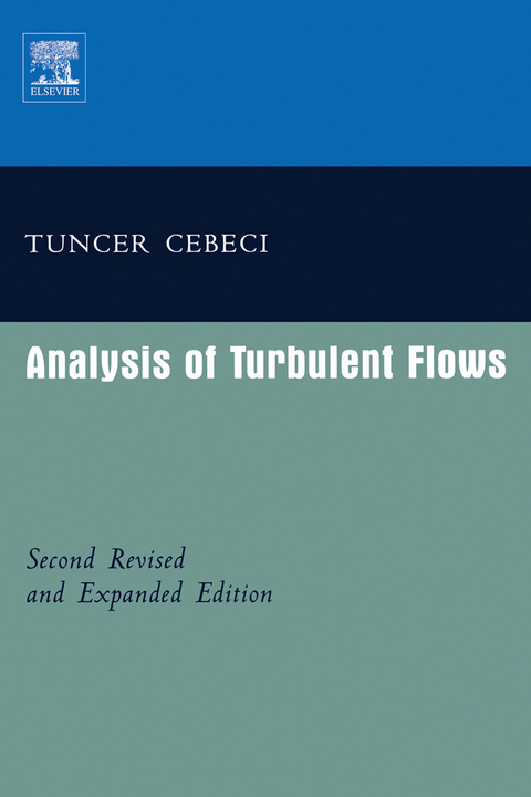
Analysis of Turbulent Flows with Computer Programs (eBook)
390 Seiten
Elsevier Science (Verlag)
978-0-08-052718-5 (ISBN)
Modelling and Computation of Turbulent Flows has been written by one of the most prolific authors in the field of CFD. Professor of aerodynamics at SUPAERO and director of DMAE at ONERA, the author calls on both his academic and industrial experience when presenting this work.
The field of CFD is strongly represented by the following corporate companies, Boeing, Airbus, Thales, United Technologies and General Electric, government bodies and academic institutions also have a strong interest in this exciting field.
Each chapter has also been specifically constructed to constitute as an advanced textbook for PhD candidates working in the field of CFD, making this book essential reading for researchers, practitioners in industry and MSc and MEng students.
* A broad overview of the development and application of Computational Fluid Dynamics (CFD), with real applications to industry
* A Free CD-Rom which contains computer program's suitable for solving non-linear equations which arise in modeling turbulent flows
* Professor Cebeci has published over 200 technical papers and 14 books, a world authority in the field of CFD
Modelling and Computation of Turbulent Flows has been written by one of the most prolific authors in the field of CFD. Professor of aerodynamics at SUPAERO and director of DMAE at ONERA, the author calls on both his academic and industrial experience when presenting this work. The field of CFD is strongly represented by the following corporate companies; Boeing; Airbus; Thales; United Technologies and General Electric, government bodies and academic institutions also have a strong interest in this exciting field. Each chapter has also been specifically constructed to constitute as an advanced textbook for PhD candidates working in the field of CFD, making this book essential reading for researchers, practitioners in industry and MSc and MEng students.* A broad overview of the development and application of Computational Fluid Dynamics (CFD), with real applications to industry* A Free CD-Rom which contains computer program's suitable for solving non-linear equations which arise in modeling turbulent flows* Professor Cebeci has published over 200 technical papers and 14 books, a world authority in the field of CFD
Front Cover 1
Analysis of Turbulent Flows 4
Copyright Page 5
Contents 10
Chapter 1. Introduction 16
1.1 Introductory Remarks 16
1.2 Turbulence–Miscellaneous Remarks 18
1.3 The Ubiquity of Turbulence 22
1.4 The Continuum Hypothesis 24
1.5 Measures of Turbulence–Intensity 25
1.6 Measures of Turbulence–Scale 29
1.7 Measures of Turbulence–The Energy Spectrum 33
1.8 Measures of Turbulence–Intermittency 35
1.9 The Diffusive Nature of Turbulence 36
1.10 Turbulence Simulation 39
References 42
Problems 44
Chapter 2. Conservation Equations for Compressible Turbulent Flows 46
2.1 Introduction 46
2.2 The Navier–Stokes Equations 46
2.3 Conventional Time-Averaging and Mass-Weighted-Averaging Procedures 48
2.4 Relation Between Conventional Time-Averaged Quantities and Mass-Weighted-Averaged Quantities 51
2.5 Continuity and Momentum Equations 53
2.6 Energy Equations 53
2.7 Mean-Kinetic-Energy Equation 54
2.8 Reynolds-Stress Transport Equations 55
2.9 Reduced Forms of the Navier–Stokes Equations 59
References 62
Problems 62
Chapter 3. Boundary-Layer Equations 64
3.1 Introduction 64
3.2 Boundary-Layer Approximations for Compressible Flows 64
3.3 Continuity, Momentum, and Energy Equations 74
3.4 Mean-Kinetic-Energy Flows 82
3.5 Reynolds-Stress Transport Equations 83
3.6 Integral Equations of the Boundary Layer 87
References 92
Problems 92
Chapter 4. General Behavior of Turbulent Boundary Layers 96
4.1 Introduction 96
4.2 Composite Nature of a Turbulent Boundary Layer 96
4.3 Eddy-Viscosity, Mixing-Length, Eddy-Conductivity and Turbulent Prandtl Number Concepts 104
4.4 Mean-Velocity and Temperature Distributions in Incompressible Flows on Smooth Surfaces 110
4.5 Mean-Velocity Distributions in Incompressible Turbulent Flows on Rough Surfaces with Zero Pressure Gradient 127
4.6 Mean-Velocity Distributions on Smooth Porous Surfaces with Zero Pressure Gradient 133
4.7 The Crocco Integral for Turbulent Boundary Layers 135
4.8 Mean-Velocity and Temperature Distributions in Compressible Flows with Zero Pressure Gradient 138
4.9 Effect of Pressure Gradient on Mean-Velocity and Temperature Distributions in Incompressible and Compressible Flows 148
References 149
Problems 151
Chapter 5. Algebraic Turbulence Models 156
5.1 Introduction 156
5.2 Eddy Viscosity and Mixing Length Models 157
5.3 CS Model 160
5.4 Extension of the CS Model to Strong Pressure -Gradient Flows 174
5.5 Extensions of the CS Model to Navier–Stokes Methods 180
5.6 Eddy Conductivity and Turbulent Prandtl Number Models 184
5.7 CS Model for Three-Dimensional Flows 191
5.8 Summary 200
References 201
Problems 205
Chapter 6.Transport-Equation Turbulence Models 208
6.1 Introduction 208
6.2 Two-Equation Models 211
6.3 One-Equation Models 222
6.4 Stress - Transport Models 225
References 228
Problems 229
Chapter 7. Short Cut Methods 232
7.1 Introduction 232
7.2 Flows with Zero-Pressure Gradient 233
7.3 Flows with Pressure Gradient: Integral Methods 251
7.4 Prediction of Flow Separation in Incompressible Flows 256
7.5 Free Shear Flows 260
Appendix 7A 273
References 275
Problems 276
Chapter 8. Differential Methods with Algebraic Turbulence Models 286
8.1 Introduction 286
8.2 Numerical Solution of the Boundary-Layer Equations with Algebraic Turbulence Models 287
8.3 Prediction of Two-Dimensional Incompressible Flows 296
8.4 Axisymmetric Incompressible Flows 305
8.5 Two-Dimensional Compressible Flows 307
8.6 Axisymmetric Compressible Flows 312
8.7 Prediction of Two-Dimensional Incompressible Flows with Separation 312
8.8 Prediction of Three-Dimensional Flows with Separation 318
References 320
Problems 322
Chapter 9. Differential Methods with Transport-Equation Turbulence Models 330
9.1 Introduction 330
9.2 Zonal Method for k-e Model 331
9.3 Solution of the k-e Model Equations with and without Wall Functions 341
9.4 Evaluation of Four Turbulence Models 345
9A. Appendix: Coefficients of the Linearized Finite-Difference Equations for the k-e Model 360
References 365
Problems 365
Chapter 10. Companion Computer Programs 376
10.1 Introduction 376
10.2 Integral Methods 376
10.3 Differential Methods with CS Model: Two-Dimensional Flows 378
10.4 Panel Method 383
10.5 Differential Method with CS Model: Two-Dimensional Flows with Heat Transfer 383
10.6 Differential Method with CS Model: Infinite Swept-Wing Flows 383
10.7 Differential Method with CS Model: Turbulent Flows with Initial Velocity Profile 384
10.8 Differential Method with SA Model 384
10.9 Differential Method for a Plane Jet 384
10.10 Useful Subroutines 384
References 386
Subject Index 388
Conservation Equations for Compressible Turbulent Flows
2.1 Introduction
In this chapter we consider the Navier-Stokes equations for a compressible fluid and show how they can be put into a form more convenient for turbulent flows. We follow the procedure first introduced by Reynolds in incompressible flows: we regard the turbulent motion as consisting of the sum of the mean part and a fluctuating part, introduce the sum into the Navier–Stokes equations, and time1 average the resulting expressions. The equations thus obtained give considerable insight into the character of turbulent motions and serve as a basis for attacking mean-flow problems, as well as for analyzing the turbulence to find its harmonic components. However, before these governing conservation equations for compressible turbulent flows are obtained, it is appropriate to write down the conservation equations for mass, momentum, and energy.
In the following sections we shall discuss the conservation equations and their reduced forms in terms of rectangular coordinates, and for convenience we shall use the summation notation. For a discussion of the conservation equations in terms of another coordinate system, the reader is referred to [1].
2.2 The Navier–Stokes Equations
The well-known Navier–Stokes equations of motion for a compressible, viscous, heat-conducting, perfect gas may be written in the following form [2]:Continuity
(2.2.1)
Momentum
(2.2.2)
Energy
(2.2.3)
wherethe stress tensor τij, heat-flux vector qj, and total enthalpy H are given by
(2.2.4)
(2.2.5)
(2.2.6)
Inthese equations, Λ is the bulk viscosity (= −2/3μ), μ the dynamic viscosity, k the thermal conductivity, and h the static enthalpy. In Eq. (2.2.4), δij is the Kronecker delta, having the value 1 for i = j and 0 for ij. A summation is understood for repeated indices.
Sometimes it is more convenient to express the energy equation in terms of static enthalpy h, rather than total enthalpy H. Then using Eqs. (2.2.1) and (2.2.2)(2.2.3) becomes
(2.2.7)
whereis the dissipation function.
Equations (2.2.1)–(2.2.7) apply to laminar as well as to turbulent flows. For the latter, however, the values of the dependent variables are to be replaced by their instantaneous values. A direct approach to the turbulence problem, namely the solution of the full time-dependent Navier–Stokes equations, then consists in solving the equations for a given set of boundary or initial values and computing mean values over the ensemble for solutions, as discussed in Section 1.10. Even for the most restricted problem – turbulence of an incompressible fluid that appears to be a hopeless undertaking, because of the nonlinear terms in the equations. Thus, the standard procedure is to average over the equations rather than over the solutions. The averaging can be done either by the conventional time-averaging procedure or by the mass-weighted averaging procedure. Both are discussed in the next section.
2.3 Conventional Time-Averaging and Mass-Weighted-Averaging Procedures
In order to obtain the governing conservation equations for turbulent flows, it is convenient to replace the instantaneous quantities in the equations of Section 2.2 by their mean and their fluctuating quantities. In the conventional time-averaging procedure, for example, the velocity and pressure are usually written in the following forms:2
(2.3.1)
(2.3.2)
whereand are the time averages of the bulk velocity and pressure, respectively, and (xi, t) and p″(xi, t) the superimposed velocity and pressure fluctuations, respectively. The time average or “mean” of any quantity q(t) is defined by
(2.3.3)
Inpractice, is taken to mean a time that is long compared to the reciprocal of the predominant frequencies in the spectrum of q; in wind-tunnel experiments, averaging times of a few seconds to a minute are usual. Clearly, the time average is useful only if it is independent of t0; a random process whose time averages are all independent of t0 is called “statistically stationary.” A nonstationary process (e.g., an air jet from a high-pressure reservoir of finite size) must be analyzed by means of “ensemble averages.” The ensemble average q is the average of a large number of instantaneous samples of q, of which one sample is taken during each run of the process at time t0 after the process starts. A process with periodicity imposed on turbulence, like the flow in a turbomachine, can be analyzed by phase averages – take averages at a given point in space over many events in which a blade is at a given position relative to that point. For further discussions, see [3].
For a fluctuating quantity q″(t), the average, , is zero, that is,
(2.3.4)
Averagevalues similar to Eqs. (2.3.1) and (2.3.2) can be written for the other flow quantities, such as density, temperature, and enthalpy, as follows:
(2.3.5)
(2.3.6)
(2.3.7)
(2.3.8)
where
As an example, let us consider the continuity and the momentum equations in the forms given by Eqs. (2.2.1) and (2.2.2), respectively, and show how they can be obtained by using the conventional time-averaging procedure for compressible turbulent flows. If we substitute the expressions given by Eqs. (2.3.1), (2.3.2), and (2.3.5) into (2.2.1) and (2.2.2) and take the time average of the terms appearing in the resulting equations, we obtain the mean continuity and the mean momentum equations in the following forms:
(2.3.9)
(2.3.10)
Forincompressible flows, d = 0. As a result Eqs. (2.3.9) and (2.3.10) can be simplified considerably; they become
(2.3.11)
(2.3.12)
We see from Eqs. (2.3.9)–(2.3.12) that the continuity and the momentum equations obtained by this procedure contain mean terms that have the same form as the corresponding terms in the instantaneous equations. However, they also have terms representing the mean effects of turbulence, which are additional unknown quantities. For that reason, the resulting conservation equations are undetermined. Consequently, the governing equations in this case, continuity and momentum, do not form a closed set. They require additional relations, which have to come from statistical or similarity considerations. The additional terms enter the governing equation as turbulent-transport terms such as and as density-generated terms such as and . In incompressible flows, the density-generated terms disappear, as is shown in Eqs. (2.3.11) and (2.3.12). In compressible flows, the continuity equation (2.3.9) has a source term, , which indicates that a mean mass interchange occurs across the mean streamlines defined in terms of ūi. It also indicates that the splitting of ui according to Eq. (2.3.1) is not convenient; it is not consistent with the usual concept of a streamline. For that reason, we shall replace the conventional time-averaging procedure by another procedure that is well known in the studies of gas mixtures, the mass-weighted-averaging procedure, which was used by Van Driest [4], Favre [5], and Laufer and Ludloff [6]. Mass-weighted averaging eliminates the mean-mass term and some of the momentum transport terms such as and across mean streamlines. We define a mass-weighted mean velocity
(2.3.13)
wherethe bar denotes conventional time averaging and the tilde denotes mass-weighted averaging. The velocity may then be written as
(2.3.14)
where(xi, t) is the superimposed velocity fluctuation. Multiplying Eq. (2.3.14) by the expression for (xi, t) given by Eq. (2.3.5) gives
Timeaveraging and noting the definition of (xi, t), we get
Fromthe definition of ūi, given by Eq. (2.3.13) it follows that
(2.3.15)
Notethe important differences between the two averaging procedures. In the conventional time averaging, in the mass-weighted averaging,
Similarly, we can define the static enthalpy, static temperature, and total enthalpy thus:
(2.3.16)
(2.3.17)
(2.3.18)
where
(2.3.19)
Also,
(2.3.20)
The expressions...
| Erscheint lt. Verlag | 20.4.2004 |
|---|---|
| Sprache | englisch |
| Themenwelt | Natur / Technik ► Fahrzeuge / Flugzeuge / Schiffe ► Luftfahrt / Raumfahrt |
| Naturwissenschaften ► Physik / Astronomie ► Angewandte Physik | |
| Naturwissenschaften ► Physik / Astronomie ► Strömungsmechanik | |
| Technik ► Bauwesen | |
| Technik ► Fahrzeugbau / Schiffbau | |
| Technik ► Luft- / Raumfahrttechnik | |
| Technik ► Maschinenbau | |
| Wirtschaft ► Betriebswirtschaft / Management ► Unternehmensführung / Management | |
| ISBN-10 | 0-08-052718-3 / 0080527183 |
| ISBN-13 | 978-0-08-052718-5 / 9780080527185 |
| Haben Sie eine Frage zum Produkt? |
Kopierschutz: Adobe-DRM
Adobe-DRM ist ein Kopierschutz, der das eBook vor Mißbrauch schützen soll. Dabei wird das eBook bereits beim Download auf Ihre persönliche Adobe-ID autorisiert. Lesen können Sie das eBook dann nur auf den Geräten, welche ebenfalls auf Ihre Adobe-ID registriert sind.
Details zum Adobe-DRM
Dateiformat: EPUB (Electronic Publication)
EPUB ist ein offener Standard für eBooks und eignet sich besonders zur Darstellung von Belletristik und Sachbüchern. Der Fließtext wird dynamisch an die Display- und Schriftgröße angepasst. Auch für mobile Lesegeräte ist EPUB daher gut geeignet.
Systemvoraussetzungen:
PC/Mac: Mit einem PC oder Mac können Sie dieses eBook lesen. Sie benötigen eine
eReader: Dieses eBook kann mit (fast) allen eBook-Readern gelesen werden. Mit dem amazon-Kindle ist es aber nicht kompatibel.
Smartphone/Tablet: Egal ob Apple oder Android, dieses eBook können Sie lesen. Sie benötigen eine
Geräteliste und zusätzliche Hinweise
Buying eBooks from abroad
For tax law reasons we can sell eBooks just within Germany and Switzerland. Regrettably we cannot fulfill eBook-orders from other countries.
aus dem Bereich


