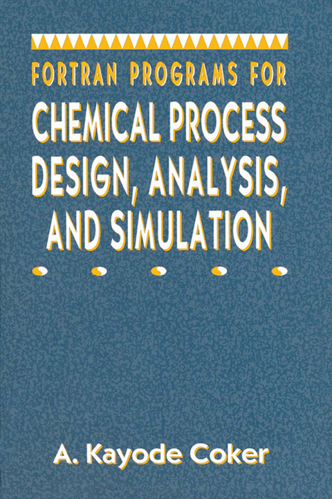
Fortran Programs for Chemical Process Design, Analysis, and Simulation (eBook)
854 Seiten
Elsevier Science (Verlag)
978-0-08-050678-4 (ISBN)
This book gives engineers the fundamental theories, equations, and computer programs (including source codes) that provide a ready way to analyze and solve a wide range of process engineering problems.
Front Cover 1
Fortran Programs for Chemical Process Design, Analysis, and Simulation 4
Copyright Page 5
Contents 6
Acknowledgment 9
Preface 10
Chapter 1. Numerical Computation 12
Chapter 2. Physical Property of Liquids and Gases 114
Chapter 3. Fluid Flow 161
Chapter 4. Equipment Sizing 267
Chapter 5. Instrument Sizing 342
Chapter 6. Compressors 431
Chapter 7. Mass Transfer 480
Chapter 8. Heat Transfer 601
Chapter 9. Engineering Economics 732
Chapter 10. The International System of Units (SI) and Conversion Tables 788
Bibliography 812
Appendix A. Tables of Selected Constants 817
Appendix B. Tables of Compressibility 833
Appendix C. Compiling the Fortran Source Code 859
Index 863
Numerical Computation
INTRODUCTION
Engineers, technologists, and scientists have employed numerical methods of analysis to solve a wide range of steady and transient problems. The fundamentals are essential in the basic operations of curve fitting, approximation, interpolation, numerical solutions of simultaneous linear and nonlinear equations, numerical differentiation and integration. These requirements are greater when new processes are designed. Engineers also need theoretical information and data from published works to construct mathematical models that simulate new processes. Developing mathematical models with personal computers sometimes involves experimental programs to obtain the required information for the models. Developing an experimental program is strongly dependent on the knowledge of the process with theory, where the whole modification can be produced by some form of mathematical models or regression analyses. Figure 1-1 shows the relationship between mathematical modeling and regression analysis.
Figure 1-1 Mathematical modeling and regression analysis. By permission, A. Constantinides, Applied Numerical Methods With Personal Computers, McGraw-Hill Book Co., 1987. McGraw-Hill
Texts [1–5] with computer programs and sometimes with supplied software are now available for scientists and engineers. They must fit a function or functions to measure data that fluctuate, which result from random error of measurement. If the number of data points equals the order of the polynomial plus one, we can exactly fit a polynomial to the data points. Fitting a function to a set of data requires more data than the order of a polynomial. The accuracy of the fitted curve depends on the large number of experimental data. In this chapter, we will develop least-squares curve fitting programs. Also, we will use linear regression analyses to develop statistical relationships involving two or more variables. The most common type of relation is a linear function. By transforming nonlinear functions, many functional relations are made linear.
For the program, we will correlate X-Y data for the following equations:
(1-1)
(1-2)
(1-3)
(1-4)
(1-5)
(1-6)
(1-7)
(1-8)
We can transform the nonlinear equations (1-5, 1-6, and 1-8) by linearizing as follows:
(1-9)
(1-10)
(1-11)
LINEAR REGRESSION ANALYSIS
Regression analysis uses statistical and mathematical methods to analyze experimental data and to fit mathematical models to these data. We can solve for the unknown parameters after fitting the model to the data. Suppose we want to find a linear function that involves paired observations on two variables, X the independent variable and Y the dependent variable. Where
n = the number of observations
Xi = the ith observation of the independent variable
Yi = the ith observation of the dependent variable
We can develop a linear regression model that expresses Y as a function of X. We can further derive formulae to determine the values of a and b that give the best fit of the equations. For each experimental point corresponding to an X-Y pair, there will be an element that represents the difference between the corresponding calculated value and the original value of Y. This is expressed as:
(1-12)
ri may be either positive or negative depending on the side of the fitted curve of X-Y points. Here, we can minimize the sum of the squares of the residuals by the following expression:
(1-13)
where
n is the number of observations of X-Y points
(1-14)
(1-15)
and
(1-16)
The problem is reduced to finding the values of a and b so that the summation of Equation 1-16 is minimized. We can obtain this by taking the partial derivative of Equation 1-16 with respect to each variable a and b and set the result to zero.
(1-17)
Substituting Equation 1-16 into Equation 1-17, we obtain
(1-18)
and
(1-19)
This is equivalent to
(1-20)
and
(1-21)
Since b, X, and Y are not functions of a, and the partial derivative of a with respect to itself is unity, Equation 1-20 reduces to
(1-22)
Similarly, a, X, and Y are not functions of b. Therefore, Equation 1-21 becomes
(1-23)
where a and b are constants. Equations 1-18 and 1-19 are expressed as:
(1-24)
and
(1-25)
We have now reduced the problem of finding a straight line through a set of X–Y data points to one of solving two simultaneous equations 1-24 and 1-25. Both equations are linear in X, Y, and n, and the unknowns a and b. Using Cramer’s rule for the simultaneous equations, we have
(1-26)
and
(1-27)
Solving Equations 1-26 and 1-27 gives
(1-28)
and
(1-29)
respectively, where all the sums are taken over all experimental observations.
Also, we can construct a table with columns headed Xi, Yi, Xi2, Xi Yi as an alternative to obtain the values of a and b. The sums of the columns will then give all the values required to Equations 1-28 and 1-29.
METHODS FOR MEASURING REGRESSION
Linear Regression
From the values of a, b, and Xi, the independent variable, we can now calculate the corresponding estimated value of Y, designated as .
(1-30)
Figure 1-2 illustrates this equation known as the regression line. The variation of the observed Y’s about the mean of the observed Y’s is the total sum of squares, and can be expressed as:
(1-31)
where
(1-32)
Figure 1-3 shows the differences between Y and , which is the total sum of squares. This is the sum of these squared differences. The total sum of squares can be expressed as:
Figure 1-2 Regression line.
Figure 1-3 Total sum of squares.
(1-33)
(1-34)
(1-35)
and since
then
(1-36)
where
(1-37)
and
(1-38)
SSE is the error (or residual) sum of squares. This is the quantity represented by Equation 1-13, that is, the equation we want to minimize. It is the sum of the differences squared between the observed Y’s and the estimated (or computed) ’s. Figure 1-4 shows the differences between the Y’s and ’s. SSR is the regression sum of squares and measures the variation of the estimated values, , about the mean of the observed Y’s and . Figure 1-5 shows the differences between Y’s and . The regression sum of squares is the sum of the squared differences.
Figure 1-4 Error sum of squares.
Figure 1-5 Regression sum of squares.
The ratio of the regression sum of squares to the total sum of squares is used in calculating the coefficient of determination. This shows how well a regression line fits the observed data. The coefficient of determination is:
(1-39)
and since SSR = SST – SSE
(1-40)
The coefficient of determination has the following properties:
1. 0 ≤ r2 ≤ 1
2. If r2 = 1 all ξi are zero. The observed Y’s and the estimated ’s are the same and this indicates a perfect fit.
3. If r2 = 0, no linear functional relationship exists.
4. As r2 approaches one, the better the fit. The closer r2 approaches zero, the worse the fit. The correlation coefficient r is:
(1-41)
Although the correlation coefficient gives a measure of the accuracy of fit, we should treat this method of analysis with great caution. Because r is close to one does not always mean that the fit is necessarily good. It is possible to obtain a high value of r when the underlying relationship between X and Y is not even linear. Draper and Smith [6] provide an excellent guidance of assessing results of linear regression.
THE ANALYSIS OF VARIANCE TABLE FOR LINEAR REGRESSION
Each sum of squares...
| Erscheint lt. Verlag | 25.1.1995 |
|---|---|
| Sprache | englisch |
| Themenwelt | Mathematik / Informatik ► Informatik ► Programmiersprachen / -werkzeuge |
| Mathematik / Informatik ► Informatik ► Theorie / Studium | |
| Informatik ► Weitere Themen ► CAD-Programme | |
| Naturwissenschaften ► Chemie ► Analytische Chemie | |
| Naturwissenschaften ► Chemie ► Technische Chemie | |
| Technik ► Umwelttechnik / Biotechnologie | |
| Wirtschaft ► Betriebswirtschaft / Management ► Logistik / Produktion | |
| Weitere Fachgebiete ► Land- / Forstwirtschaft / Fischerei | |
| ISBN-10 | 0-08-050678-X / 008050678X |
| ISBN-13 | 978-0-08-050678-4 / 9780080506784 |
| Informationen gemäß Produktsicherheitsverordnung (GPSR) | |
| Haben Sie eine Frage zum Produkt? |
Kopierschutz: Adobe-DRM
Adobe-DRM ist ein Kopierschutz, der das eBook vor Mißbrauch schützen soll. Dabei wird das eBook bereits beim Download auf Ihre persönliche Adobe-ID autorisiert. Lesen können Sie das eBook dann nur auf den Geräten, welche ebenfalls auf Ihre Adobe-ID registriert sind.
Details zum Adobe-DRM
Dateiformat: PDF (Portable Document Format)
Mit einem festen Seitenlayout eignet sich die PDF besonders für Fachbücher mit Spalten, Tabellen und Abbildungen. Eine PDF kann auf fast allen Geräten angezeigt werden, ist aber für kleine Displays (Smartphone, eReader) nur eingeschränkt geeignet.
Systemvoraussetzungen:
PC/Mac: Mit einem PC oder Mac können Sie dieses eBook lesen. Sie benötigen eine
eReader: Dieses eBook kann mit (fast) allen eBook-Readern gelesen werden. Mit dem amazon-Kindle ist es aber nicht kompatibel.
Smartphone/Tablet: Egal ob Apple oder Android, dieses eBook können Sie lesen. Sie benötigen eine
Geräteliste und zusätzliche Hinweise
Buying eBooks from abroad
For tax law reasons we can sell eBooks just within Germany and Switzerland. Regrettably we cannot fulfill eBook-orders from other countries.
aus dem Bereich


