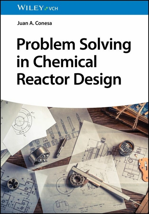
Problem Solving in Chemical Reactor Design (eBook)
691 Seiten
Wiley-VCH (Verlag)
978-3-527-84801-0 (ISBN)
Extensive workbook with more than 200 up-to-date solved problems on advanced chemical reactors for deeper understanding of chemical reactor design
Problem Solving in Chemical Reactor Design provides in-depth coverage of more than 200 solved complex reactor design problems extracted from core chemical engineering subject areas. The problems in this book cover the design of non-ideal, catalytic, multiphase, heterogeneous, and biochemical reactors rather than focusing on basic Chemical Reactor Engineering concepts.
Each complex problem is solved using simple procedures and mathematical tools, enabling readers to better understand the correct procedure for solving problems and solve them faster, more conveniently, and more accurately.
This book is inspired by more than two decades of the author's teaching experience in chemical reactor engineering. Accompanying electronic materials include spreadsheets and easily understandable Matlab® programs, which can both be downloaded from the Wiley website.
Some of the topics covered in Problem Solving in Chemical Reactor Design include:
- Optimization, operation, and complexities of reactor design in the face of non-idealities such as mixing issues and residence time distributions
- Utilization of the tanks-in-series model, dispersion model, and intricate combinations of ideal reactors to elucidate the impact on conversion rates
- Signal processing within the domain of chemical reactor engineering, specifically focusing on convolution and deconvolution methodologies
- Reaction kinetics, diffusion dynamics, and catalyst efficiency in catalytic reactor design, and design of gas-catalytic and gas-liquid-solid catalyst systems in multiphase reactors
Problem Solving in Chemical Reactor Design is an excellent learning resource for students and professionals in the fields of chemical engineering, pharmaceuticals, biotechnology, and fine chemistry.
Juan A. Conesa, PhD, is a distinguished Professor of Chemical Engineering at the University of Alicante, Spain. With over 30 years of experience, his research focuses on decomposition kinetics, waste degradation, and pollutant analysis under various conditions. He is particularly renowned for his work on dioxins and furans analysis in waste treatment processes. Since 2015, he has led the research group 'Waste, Energy, Environment and Nanotechnology (WEEN)' at the University of Alicante.
1
Non-ideal Flow and Reactor Characterization
Summary of Residence Time Distribution Properties and Most Important Models
Residence Time Distribution
In a reactor, C(t) is obtained by injecting pulse of tracer. From that:
Total amount of tracer injected is:
In a step tracer run:
Mean residence time:
Variance of the residence time distribution (RTD):
The square root of the variance, σ, is called standard deviation.
Average residence time:
RTD in Ideal Reactors
For the plug flow reactor (PFR):
For the continuous stirred tank reactor (CSTR):
Tanks-in-series (TIS) Model
Dispersion Model
Bo < 0.01
Bo > 0.01, Closed–Closed Recipient
E(t) is only integrable by numerical methods.
Bo > 0.01, Open–Open Recipient
Designing E1 to the E(t) given by the first expression (valid for Bo < 0.01) and E2 to the one predicted by the open–open (o–o) assumption, the differences between these RTDs are small at low Bo, but at a high Bo number, E1 is not valid (for more details, consult spreadsheet “dispersion model Bo fitting.xls”):
Problem 1.1 A solution of potassium permanganate (KMnO4) was rapidly injected into a water stream flowing through a circular tube at a linear velocity of 35.70 cm/s. A photoelectric cell located 2.74 m downstream from the injection point was utilized to monitor the local concentration of KMnO4.
- (a) By using the given effluent KMnO4 concentrations, calculate the average residence time of the fluid as well as the variance, E(t), F(t), and I(t).
- (b) Determine the number of ideal tanks (nt), the variance, the dispersion number, and the Peclet number.
| Time (s) | KMnO4 concentration |
|---|
| 0.0 | 0.0 |
| 2.0 | 11.0 |
| 4.0 | 53.0 |
| 6.0 | 64.0 |
| 8.0 | 58.0 |
| 10.0 | 48.0 |
| 12.0 | 39.0 |
| 14.0 | 29.0 |
| 16.0 | 22.0 |
| 18.0 | 16.0 |
| 20.0 | 11.0 |
| 22.0 | 9.0 |
| 24.0 | 7.0 |
| 26.0 | 5.0 |
| 28.0 | 4.0 |
| 30.0 | 2.0 |
| 32.0 | 2.0 |
| 34.0 | 2.0 |
| 36.0 | 1.0 |
| 38.0 | 1.0 |
| 40.0 | 1.0 |
| 42.0 | 1.0 |
Solution to Problem 1.1
For details refer the Wiley website at http://www.wiley-vch.de/ISBN9783527354115
- (a) To solve this problem, we should use a spreadsheet. First, data given in the statement are introduced, and then we should do the following calculations:
t (s) C(t) C(t)dt E(t) t·E(t) t·E(t)·Δt (t − tm)2·E(t) (t − tm)2·E(t)·Δt F(t) I(t) 0 0 0 0.000 0.000 0.000 0.000 0.000 0.000 1.000 2 11 11 0.014 0.029 0.029 1.149 1.149 0.029 0.971 4 53 64 0.069 0.275 0.304 3.345 4.494 0.166 0.834 6 64 117 0.083 0.498 0.773 2.055 5.399 0.332 0.668 8 58 122 0.075 0.602 1.100 0.666 2.721 0.482 0.518 10 48 106 0.062 0.623 1.224 0.059 0.725 0.607 0.393 12 39 87 0.051 0.607 1.230 0.053 0.112 0.708 0.292 14 29 68 0.038 0.527 1.134 0.344 0.397 0.783 0.217 16 22 51 0.029 0.457 0.983 0.720 1.065 0.840 0.160 18 16 38 0.021 0.374 0.830 1.024 1.744 0.882 0.118 20 11 27 0.014 0.285 0.659 1.162 2.186 0.911 0.089 22 9 20 0.012 0.257 0.542 1.419 2.581 0.934 0.066 24 7 16 0.009 0.218 0.475 1.540 2.959 0.952 0.048 26 5 12 0.006 0.169 0.387 1.464 3.004 0.965 0.035 28 4 9 0.005 0.145 0.314 1.504 2.968 0.975 0.025 30 2 6 0.003 0.078 0.223 0.939 2.443 0.981 0.019 32 2 4 0.003 0.083 0.161 1.147 2.086 0.986 0.014 34 2 4 0.003 0.088 0.171 1.375 2.522 0.991 0.009 36 1 3 0.001 0.047 0.135 0.812 2.187 0.994 0.006 38 1 2 0.001 0.049 0.096 0.947 1.759 0.996 0.004 40 1 2 0.001 0.052 0.101 1.093 2.040 0.999 0.001 42 1 2 0.001 0.054 0.106 1.248 2.341 Σ(C(t)dt) = 771tm = 10.98 sσ2 = 46.88 s2 We can calculate time increment as the difference between time in two experimental data; in the third column, concentration and time increment are multiplied. For a better calculation, instead of calculating C(t)·Δt for each time directly, we can use the average value of C(t) between two consecutive data. This is called Simpson’s rule for evaluating areas graphically. The sum of the values in this column would give the area of the C(t) curve, so in the fourth column, the following relationship is applied to calculate E(t):
In the next columns, the average value of E(t) between two consecutive data is multiplied by time, by time increment, and the sum would represent mean time, as we have:
In a similar way, variance is calculated:
Finally, we can calculate F(t) and I(t) according to their definitions:
We can check the form of the graphs showing the distributions:
- (b) From the calculated parameters, it is easy to find the number of tanks in the TIS model:
For the dispersion model to be applied, first we should assume Bo < 0.01, and then:
We obtain Bo = 11.24 ≫ 0.01, so this assumption is not valid.
Assuming now...
| Erscheint lt. Verlag | 4.9.2024 |
|---|---|
| Sprache | englisch |
| Themenwelt | Naturwissenschaften ► Chemie |
| Schlagworte | biochemical reactors • Catalyst Systems • catalytic reactors • Chemical Reactor Engineering • Heterogeneous Reactors • Multiphase Reactors • non-ideal reactors • Reaction kinetics • Reactor Design • reactor operation • reactor optimization |
| ISBN-10 | 3-527-84801-0 / 3527848010 |
| ISBN-13 | 978-3-527-84801-0 / 9783527848010 |
| Informationen gemäß Produktsicherheitsverordnung (GPSR) | |
| Haben Sie eine Frage zum Produkt? |
Kopierschutz: Adobe-DRM
Adobe-DRM ist ein Kopierschutz, der das eBook vor Mißbrauch schützen soll. Dabei wird das eBook bereits beim Download auf Ihre persönliche Adobe-ID autorisiert. Lesen können Sie das eBook dann nur auf den Geräten, welche ebenfalls auf Ihre Adobe-ID registriert sind.
Details zum Adobe-DRM
Dateiformat: EPUB (Electronic Publication)
EPUB ist ein offener Standard für eBooks und eignet sich besonders zur Darstellung von Belletristik und Sachbüchern. Der Fließtext wird dynamisch an die Display- und Schriftgröße angepasst. Auch für mobile Lesegeräte ist EPUB daher gut geeignet.
Systemvoraussetzungen:
PC/Mac: Mit einem PC oder Mac können Sie dieses eBook lesen. Sie benötigen eine
eReader: Dieses eBook kann mit (fast) allen eBook-Readern gelesen werden. Mit dem amazon-Kindle ist es aber nicht kompatibel.
Smartphone/Tablet: Egal ob Apple oder Android, dieses eBook können Sie lesen. Sie benötigen eine
Geräteliste und zusätzliche Hinweise
Buying eBooks from abroad
For tax law reasons we can sell eBooks just within Germany and Switzerland. Regrettably we cannot fulfill eBook-orders from other countries.
aus dem Bereich


