Theodoros Giannakopoulos is a Research Associate in the Institute of Informatics and Telecommunications, National Center for Scientific Research DEMOKRITOS, Greece and in the Department of Informatics & Telecommunications of the University of Athens (UOA). He received his Ph.D. degree in Audio Analysis from UOA, in 2009. His main research interests are pattern recognition, data mining, and multimedia analysis.
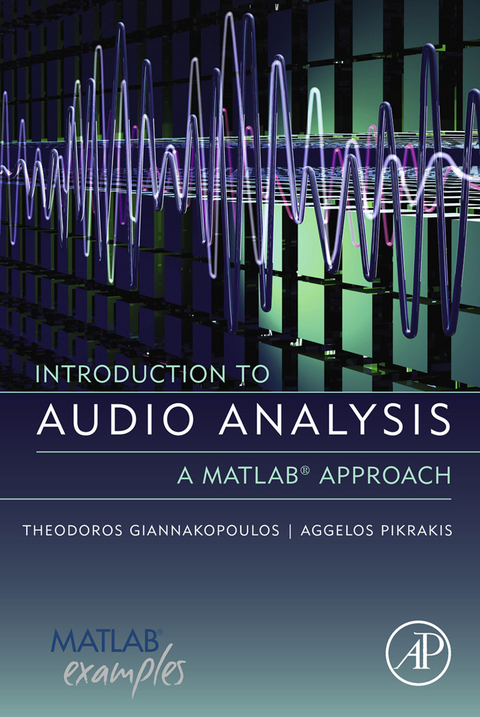
Introduction to Audio Analysis serves as a standalone introduction to audio analysis, providing theoretical background to many state-of-the-art techniques. It covers the essential theory necessary to develop audio engineering applications, but also uses programming techniques, notably MATLAB(R), to take a more applied approach to the topic. Basic theory and reproducible experiments are combined to demonstrate theoretical concepts from a practical point of view and provide a solid foundation in the field of audio analysis. Audio feature extraction, audio classification, audio segmentation, and music information retrieval are all addressed in detail, along with material on basic audio processing and frequency domain representations and filtering. Throughout the text, reproducible MATLAB examples are accompanied by theoretical descriptions, illustrating how concepts and equations can be applied to the development of audio analysis systems and components. A blend of reproducible MATLAB code and essential theory provides enable the reader to delve into the world of audio signals and develop real-world audio applications in various domains. - Practical approach to signal processing: The first book to focus on audio analysis from a signal processing perspective, demonstrating practical implementation alongside theoretical concepts- Bridge the gap between theory and practice: The authors demonstrate how to apply equations to real-life code examples and resources, giving you the technical skills to develop real-world applications- Library of MATLAB code: The book is accompanied by a well-documented library of MATLAB functions and reproducible experiments
List of Figures
| Figure 2.1 | A synthetic audio signal. | 12 |
| Figure 2.2 | A STEREO audio signal. | 14 |
| Figure 2.3 | Short-term processing of an audio signal. | 26 |
| Figure 3.1 | Plots of the magnitude of the spectrum of a signal consisting of three frequencies at 200, 500, and 1200 Hz. | 38 |
| Figure 3.2 | A synthetic signal consisting of three frequencies is corrupted by additive noise. | 40 |
| Figure 3.3 | The spectrogram of a speech signal. | 41 |
| Figure 3.4 | Spectrograms of a synthetic, frequency-modulated signal for three short-term frame lengths. | 42 |
| Figure 3.5 | Spectrum representations of (a) an analog signal, (b) a sampled version when the sampling frequency exceeds the Nyquist rate, and (c) a sampled version with insufficient sampling frequency. In the last case, the shifted versions of the analog spectrum are overlapping, hence the aliasing effect. | 43 |
| Figure 3.6 | Spectral representations of the same three-tone (200, 500 and 3000 HZ) signal for two different sampling frequencies (8 kHz and 4 kHz). | 44 |
| Figure 3.7 | Frequency response of a pre-emphasis filter for a = −0.95. | 51 |
| Figure 3.8 | An example of the application of a lowpass filter on a synthetic signal consisting of three tones. | 53 |
| Figure 3.9 | Example of a simple speechdenoising technique applied on a segment of the diarizationExample.wav file, found in the data folder of the library of the book. | 55 |
| Figure 4.1 | Mid-term feature extraction: each mid-term segment is short-term processed and statistics are computed based on the extracted feature sequence. | 63 |
| Figure 4.2 | Plotting the results of featureExtractionFile(), using plotFeaturesFile(), for the six feature statistics drawn from the 6th adopted audio feature. | 68 |
| Figure 4.3 | Histograms of the standard deviation by mean ratio of the short-term energy for two classes: music and speech. | 72 |
| Figure 4.4 | Example of a speech segment and the respective sequence of ZCR values. | 74 |
| Figure 4.5 | Histograms of the standard deviation of the ZCR for music and speech classes. | 75 |
| Figure 4.6 | Sequence of entropy values for an audio signal that contains the sounds of three gunshots. Low values appear at the onset of each gunshot. | 77 |
| Figure 4.7 | Histograms of the minimum value of the entropy of energy for audio segments from the genres of jazz, classical and electronic music. | 78 |
| Figure 4.8 | Histograms of the maximum value of the sequence of values of the spectral centroid, for audio segments from three classes of environmental sounds: others1, others2, and others3. | 81 |
| Figure 4.9 | Histograms of the maximum value of the sequences of the spectral spread feature, for audio segments from three music genres: classical, jazz, and electronic. | 82 |
| Figure 4.10 | Histograms of the standard deviation of sequences of the spectral entropy feature, for audio segments from three classes: music, speech, and others1 (low-level environmental sounds). | 83 |
| Figure 4.11 | Histograms of the mean value of the sequence of spectral flux values, for audio segments from two classes: music and speech. | 85 |
| Figure 4.12 | Example of the spectral rolloff sequence of an audio signal that consists of four music excerpts. The first 5 s stem from a classical music track. | 87 |
| Figure 4.13 | Frequency warping function for the computation of the MFCCs. | 88 |
| Figure 4.14 | Histograms of the standard deviation of the 2nd MFCC for the classes of music and speech. | 91 |
| Figure 4.15 | Chromagrams for a music and a speech segment. | 92 |
| Figure 4.16 | Autocorrelation, normalized autocorrelation, and detected peak for a periodic signal. | 94 |
| Figure 4.17 | Histograms of the maximum value of sequences of values of the harmonic ratio for two classes of sounds (speech and others1). | 96 |
| Figure 5.1 | Generic diagram of the classifier training stage. | 112 |
| Figure 5.2 | Diagram of the classification process. | 113 |
| Figure 5.3 | Linearly separable classes in a two-dimensional feature space. | 118 |
| Figure 5.4 | Decision tree for a classification task with 3-classes (ω1, ω2, ω3) and three features (x1, x2, x3). | 122 |
| Figure 5.5 | Decision tree for a 4-class task with Gaussian feature distributions in the two-dimensional feature space. | 123 |
| Figure 5.6 | Decision tree for amusical genre classification taskwith two feature statistics (minimum value of the entropy of energy and mean value of the spectral flux). | 124 |
| Figure 5.7 | SVM training for different values of the C parameter. | 128 |
| Figure 5.8 | Classification accuracy on the training andtestingdataset for different values of C. | 129 |
| Figure 5.9 | Implementation of the k-NN classification procedure. | 132 |
| Figure 5.10 | Binary classification task with Gaussian feature distributions and two different decision thresholds. | 137 |
| Figure 5.11 | Performance of the k-NN classifier on an 8-class task, for different values of the k parameter and for two validation methods (repeated hold-out and leave-one-out). | 143 |
| Figure 5.12 | Estimated performance for the 3-class musical genre classification task, for different values of the k parameter and for two evaluation methods (repeated hold-out and leave-one-out). | 145 |
| Figure 6.1 | Post-segmentation stage: the output of the first stage can be (a) a sequence of hard classification decisions, Ci i =1, …, Nmt; or (b) a sequence of sets of posterior probability estimates, Pi(j), i = 1,…, Nmt, j = 1,…,Nc. | 155 |
| Figure 6.2 | Fixed-window segmentation. | 156 |
| Figure 6.3 | Fixed-window segmentation: naive merging vs Viterbi-based smoothing. | 159 |
| Figure 6.4 | Example of the silence detection approach implemented in silenceDetectorUtterance(). | 162 |
| Figure 6.5 | Speech-silence segmenter applied on a short-duration signal. | 164 |
| Figure 6.6 | Fixed-window segmentation with an embedded 4-class classifier (silence, male speech, female speech, and music). | 166 |
| Figure 6.7 | A sequence of segments in the dynamic programming grid. | 168 |
| Figure 6.8 | Top: Signal change detection results from a TV program. Bottom: Ground truth. | 171 |
| Figure 6.9 | A clustering example in the two-dimensional feature space. | 173 |
| Figure 6.10 | Silhouette example: the average Silhouette measure is maximized when the number of clusters is 4. | 176 |
| Figure... |
| Erscheint lt. Verlag | 15.2.2014 |
|---|---|
| Sprache | englisch |
| Themenwelt | Mathematik / Informatik ► Informatik ► Programmiersprachen / -werkzeuge |
| Naturwissenschaften ► Physik / Astronomie ► Elektrodynamik | |
| Technik ► Bauwesen | |
| Technik ► Elektrotechnik / Energietechnik | |
| ISBN-10 | 0-08-099389-3 / 0080993893 |
| ISBN-13 | 978-0-08-099389-8 / 9780080993898 |
| Haben Sie eine Frage zum Produkt? |
Größe: 21,0 MB
Kopierschutz: Adobe-DRM
Adobe-DRM ist ein Kopierschutz, der das eBook vor Mißbrauch schützen soll. Dabei wird das eBook bereits beim Download auf Ihre persönliche Adobe-ID autorisiert. Lesen können Sie das eBook dann nur auf den Geräten, welche ebenfalls auf Ihre Adobe-ID registriert sind.
Details zum Adobe-DRM
Dateiformat: PDF (Portable Document Format)
Mit einem festen Seitenlayout eignet sich die PDF besonders für Fachbücher mit Spalten, Tabellen und Abbildungen. Eine PDF kann auf fast allen Geräten angezeigt werden, ist aber für kleine Displays (Smartphone, eReader) nur eingeschränkt geeignet.
Systemvoraussetzungen:
PC/Mac: Mit einem PC oder Mac können Sie dieses eBook lesen. Sie benötigen eine
eReader: Dieses eBook kann mit (fast) allen eBook-Readern gelesen werden. Mit dem amazon-Kindle ist es aber nicht kompatibel.
Smartphone/Tablet: Egal ob Apple oder Android, dieses eBook können Sie lesen. Sie benötigen eine
Geräteliste und zusätzliche Hinweise
Buying eBooks from abroad
For tax law reasons we can sell eBooks just within Germany and Switzerland. Regrettably we cannot fulfill eBook-orders from other countries.
Größe: 6,8 MB
Kopierschutz: Adobe-DRM
Adobe-DRM ist ein Kopierschutz, der das eBook vor Mißbrauch schützen soll. Dabei wird das eBook bereits beim Download auf Ihre persönliche Adobe-ID autorisiert. Lesen können Sie das eBook dann nur auf den Geräten, welche ebenfalls auf Ihre Adobe-ID registriert sind.
Details zum Adobe-DRM
Dateiformat: EPUB (Electronic Publication)
EPUB ist ein offener Standard für eBooks und eignet sich besonders zur Darstellung von Belletristik und Sachbüchern. Der Fließtext wird dynamisch an die Display- und Schriftgröße angepasst. Auch für mobile Lesegeräte ist EPUB daher gut geeignet.
Systemvoraussetzungen:
PC/Mac: Mit einem PC oder Mac können Sie dieses eBook lesen. Sie benötigen eine
eReader: Dieses eBook kann mit (fast) allen eBook-Readern gelesen werden. Mit dem amazon-Kindle ist es aber nicht kompatibel.
Smartphone/Tablet: Egal ob Apple oder Android, dieses eBook können Sie lesen. Sie benötigen eine
Geräteliste und zusätzliche Hinweise
Buying eBooks from abroad
For tax law reasons we can sell eBooks just within Germany and Switzerland. Regrettably we cannot fulfill eBook-orders from other countries.
aus dem Bereich


