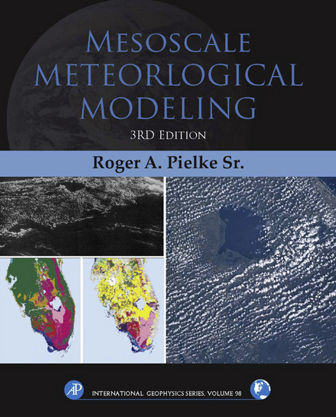
The 3rd edition of Mesoscale Meteorological Modeling is a fully revised resource for researchers and practitioners in the growing field of meteorological modeling at the mesoscale. Pielke has enhanced the new edition by quantifying model capability (uncertainty) by a detailed evaluation of the assumptions of parameterization and error propagation. Mesoscale models are applied in a wide variety of studies, including weather prediction, regional and local climate assessments, and air pollution investigations. - Broad expansion of the concepts of parameterization and parameterization methodology- Addition of new modeling approaches, including modeling summaries and summaries of data sets- All-new section on dynamic downscaling
Simplification of the Basic Equations
Roger A. Pielke Sr.
Abstract
This chapter discusses how the fundamental conservation equations can be simplified using scale analysis. These simplifications can result in the conversion of a prognostic conservation equation to a diagnostic equation. Such simplifications are used, for example, to create the replacement of the vertical equation-of-motion with the hydrostatic, and the replacement of the prognostic equation for mass with the anelastic and incompressible so-called “continuity” equations.
Keywords
Scale analysis; deep continuity equation; shallow continuity equation; hydrostatic relationship; geostrophic wind; gradient wind; Reynolds number; Coriolis parameter
Equations 2.43–2.47 can be simplified for specific mesoscale meteorological simulations, and by mathematical operations, some of these relations can also be changed in form. In this chapter, commonly made assumptions will be reviewed and the resultant equations presented. In all cases, the Eqs. 2.43–2.47 are altered in form or simplified, or both, to permit their solutions to be made in an easier, more economical fashion.
The method of scale analysis1 is often used to determine the relative importance of the individual terms in the conservation relations. This technique involves the estimation of their order of magnitude through the use of representative values of the dependent variables and constants that make up these terms. Scale analysis can be applied either to individual terms in the fundamental conservation equations, as applied in this chapter, or to analytic solutions of a coupled set of the conservation equations, as discussed in Section 5.2.2. The most rigorous analysis procedure, of course, is to evaluate specific solutions of the conservation equations with and without particular terms to establish their importance. An example of such an analysis for the hydrostatic assumption in sea-breeze simulations, is described in Section 5.2.3.
In this chapter, the use of scale analysis is summarized. Discussions by investigators such as Thunis and Bornstein (1996) provide additional descriptions of the use of scale analysis to investigate scales of motion on the mesoscale.
3.1 Conservation of Mass
In Chapter 2, the mass-conservation relation was given by Eq. 2.43. To determine appropriate and consistent approximate forms of this equation, portions of the scale analysis of this equation by Dutton and Fichtl (1969) are utilized in the following discussion.
Using the relationship between density and specific volume given by
Eq. 2.43 can be rewritten as
(3.1)
If it is assumed that
where is defined as a synoptic-scale reference specific volume and is the mesoscale perturbation from this value,2 then Eq. 3.1 can be rewritten as
(3.2)
To simplify the scale analysis of this equation, it is assumed that
(3.3)
so that Eq. 3.2 becomes
(3.4)
For mesoscale atmospheric circulations, the adoption of the assumptions given in Eq. 3.3 requires that the synoptic state change much more slowly than the mesoscale system and that the horizontal synoptic gradients are much less than the mesoscale gradients.
It is also assumed that
so that Eq. 3.4 reduces to
(3.5)
This requirement on the ratio of the mesoscale perturbation specific volume to the synoptic-scale reference value is reasonable when realistic values of temperature and pressure are inserted into the ideal gas law (Eq. 2.13).
For example, a representative climatological value of at sea level is . Since , upper and lower bounds on specific volume can be estimated for realistic mesoscale situations using the highest temperature and lowest pressure and the lowest temperature and highest pressure likely to occur at a given location over a reasonably short time period (say 12-24 h). If
and
then and for the two cases, so that is at most around .
The method of scale analysis is used to estimate the magnitude of the remaining terms in Eq. 3.5, so that
(3.6)
where represents the characteristic frequency of variations in specific volume on the mesoscale; , and are representative values of the components of velocity; , and are the spatial scales of the mesoscale disturbance; and , the density-scaled height of the atmosphere, is defined as
In the Earth’s troposphere, is approximately 8 km, as illustrated schematically in Fig. 3.1.
Figure 3.1 Schematic illustration contrasting deep and shallow atmospheric circulations. The depth corresponds to the vertical extent of the circulation. In the Earth’s atmosphere, .
3.1.1 Deep Continuity Equation
To examine the necessity for retaining individual terms in Eq. 3.5, it is customary to examine their ratio relative to one of the terms that is expected to remain. In the first case to be examined, the terms are divided by the order of magnitude estimate for , resulting in
Since , the terms , and are much less than , and and can be neglected in Eq. 3.5, provided
(3.7)
Then Eq. 3.5 can be written as
(3.8)
Since is approximately equal to , conditions (ii) and (iii) in Eq. 3.7 require that
(3.9)
If therefore, is one or two orders of magnitude larger than , it is expected that the vertical velocity should be one or two orders of magnitude less than and (e.g., for , then ). This relation between velocities and the horizontal and vertical scales of atmospheric circulations results from the condition that . Because of this constraint, velocities in a longer, horizontal leg of an atmospheric circulation must be proportionately stronger to preserve mass continuity without creating large fluctuations in specific volume.
The last requirement that needs to be justified in Eq. 3.7 is condition (iv). The scaled variable represents a time period in which significant variations in specific volume occur on the mesoscale and can be approximated by
(3.10)
where is the wavelength over which variations occur and the rate of movement of these variations. If the changes are caused by advection, then , or is used to represent , whereas a characteristic group velocity will be utilized if wave propagation is dominant. The wavelength is estimated as and for horizontal motion and for vertical movement. When changes in specific volume are assumed primarily to be caused by advection or when the wave group velocity has approximately the same speed as the wind velocity,3 then
where conditions (i)-(iii) in Eq. 3.7 have been used. Therefore,
so that local variations in density can be neglected in the conservation of mass relation if .
Finally, if , mesoscale variations in the direction are expected to be dominant and the derivatives in Eq. 3.8 can be ignored. In this case the equation reduces to the two-dimensional form given by
Equation 3.8 is customarily written to include the terms and and is given by
or, returning to the use of density instead of specific volume,
(3.11)
where .
Dutton and Fichtl (1969) refer to this relation as the deep convection continuity equation because the vertical depth of the circulation is on the same order as the density scale depth. As originally shown by Ogura and Phillips (1962), and discussed by Lipps and Hemler (1982), and as will be shown in Section 5.2.2, the use of this form of the conservation-of-mass relation eliminates sound waves as a possible solution, which led Ogura and Phillips to refer to Eq. 3.11 as the anelastic, or soundproof assumption. Because such waves are of no direct interest in most applications of mesoscale meteorology, this equation is often employed to represent mass conservation in mesoscale models in lieu of the more complete prognostic conservation-of-mass equation given by Eq. 3.1. Moreover, as discussed in Section 9.3, the elimination of sound waves permits more economical use of certain numerical solution techniques because their computational stability is dependent on having a time step less than or equal to the time it takes a wave to travel between grid points. Sound waves are the fastest nonelectromagnetic waveform in the atmosphere.
3.1.2 Shallow Continuity Equation
A more restrictive mass-conservation relation is derived by dividing the scaled terms in Eq. 3.6 by the scaled form of resulting in
As in the previous analysis, since , and can be neglected in Eq. 3.5, provided
(3.12)
then Eq. 3.5 can be written as
(3.13)
The first condition in Eq. 3.12 is easier to satisfy than the equivalent requirement in Eq. 3.7 because . This requirement implies that the neglect of specific volume variations in Eq. 3.13 is even less important than in Eq. 3.11. The second condition in Eq. 3.12 requires that the depth of the circulation be much less than the scale depth of the atmosphere. For this reason Dutton and Fichtl refer to Eq. 3.13 as the shallow convection continuity equation. Written in tensor...
| Erscheint lt. Verlag | 8.10.2013 |
|---|---|
| Sprache | englisch |
| Themenwelt | Mathematik / Informatik ► Informatik |
| Mathematik / Informatik ► Mathematik ► Angewandte Mathematik | |
| Naturwissenschaften ► Biologie ► Ökologie / Naturschutz | |
| Naturwissenschaften ► Geowissenschaften ► Meteorologie / Klimatologie | |
| Naturwissenschaften ► Physik / Astronomie ► Angewandte Physik | |
| Technik ► Bauwesen | |
| Technik ► Umwelttechnik / Biotechnologie | |
| ISBN-10 | 0-12-385238-2 / 0123852382 |
| ISBN-13 | 978-0-12-385238-0 / 9780123852380 |
| Informationen gemäß Produktsicherheitsverordnung (GPSR) | |
| Haben Sie eine Frage zum Produkt? |
Größe: 32,1 MB
Kopierschutz: Adobe-DRM
Adobe-DRM ist ein Kopierschutz, der das eBook vor Mißbrauch schützen soll. Dabei wird das eBook bereits beim Download auf Ihre persönliche Adobe-ID autorisiert. Lesen können Sie das eBook dann nur auf den Geräten, welche ebenfalls auf Ihre Adobe-ID registriert sind.
Details zum Adobe-DRM
Dateiformat: PDF (Portable Document Format)
Mit einem festen Seitenlayout eignet sich die PDF besonders für Fachbücher mit Spalten, Tabellen und Abbildungen. Eine PDF kann auf fast allen Geräten angezeigt werden, ist aber für kleine Displays (Smartphone, eReader) nur eingeschränkt geeignet.
Systemvoraussetzungen:
PC/Mac: Mit einem PC oder Mac können Sie dieses eBook lesen. Sie benötigen eine
eReader: Dieses eBook kann mit (fast) allen eBook-Readern gelesen werden. Mit dem amazon-Kindle ist es aber nicht kompatibel.
Smartphone/Tablet: Egal ob Apple oder Android, dieses eBook können Sie lesen. Sie benötigen eine
Geräteliste und zusätzliche Hinweise
Zusätzliches Feature: Online Lesen
Dieses eBook können Sie zusätzlich zum Download auch online im Webbrowser lesen.
Buying eBooks from abroad
For tax law reasons we can sell eBooks just within Germany and Switzerland. Regrettably we cannot fulfill eBook-orders from other countries.
Größe: 30,3 MB
Kopierschutz: Adobe-DRM
Adobe-DRM ist ein Kopierschutz, der das eBook vor Mißbrauch schützen soll. Dabei wird das eBook bereits beim Download auf Ihre persönliche Adobe-ID autorisiert. Lesen können Sie das eBook dann nur auf den Geräten, welche ebenfalls auf Ihre Adobe-ID registriert sind.
Details zum Adobe-DRM
Dateiformat: EPUB (Electronic Publication)
EPUB ist ein offener Standard für eBooks und eignet sich besonders zur Darstellung von Belletristik und Sachbüchern. Der Fließtext wird dynamisch an die Display- und Schriftgröße angepasst. Auch für mobile Lesegeräte ist EPUB daher gut geeignet.
Systemvoraussetzungen:
PC/Mac: Mit einem PC oder Mac können Sie dieses eBook lesen. Sie benötigen eine
eReader: Dieses eBook kann mit (fast) allen eBook-Readern gelesen werden. Mit dem amazon-Kindle ist es aber nicht kompatibel.
Smartphone/Tablet: Egal ob Apple oder Android, dieses eBook können Sie lesen. Sie benötigen eine
Geräteliste und zusätzliche Hinweise
Zusätzliches Feature: Online Lesen
Dieses eBook können Sie zusätzlich zum Download auch online im Webbrowser lesen.
Buying eBooks from abroad
For tax law reasons we can sell eBooks just within Germany and Switzerland. Regrettably we cannot fulfill eBook-orders from other countries.
aus dem Bereich


