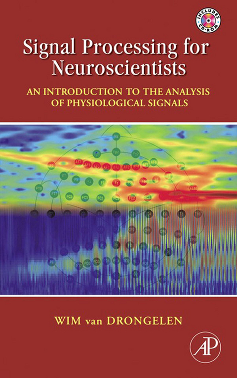
Signal Processing for Neuroscientists (eBook)
320 Seiten
Elsevier Science (Verlag)
978-0-08-046775-7 (ISBN)
Wim van Drongelen studied Biophysics at the University Leiden, The Netherlands. After a period in the Laboratoire d'Electrophysiologie, Université Claude Bernard, Lyon, France, he received the Doctoral degree cum laude. In 1980 he received the Ph.D. degree. He worked for the Netherlands Organization for the Advancement of Pure Research (ZWO) in the Department of Animal Physiology, Wageningen, The Netherlands. He lectured and founded a Medical Technology Department at the HBO Institute Twente, The Netherlands. In 1986 he joined the Benelux office of Nicolet Biomedical as an Application Specialist and in 1993 he relocated to Madison, WI, USA where he was involved in research and development of equipment for clinical neurophysiology and neuromonitoring. In 2001 he joined the Epilepsy Center at The University of Chicago, Chicago, IL, USA. Currently he is Professor of Pediatrics, Neurology, and Computational Neuroscience. In addition to his faculty position he serves as Technical and Research Director of the Pediatric Epilepsy Center and he is Senior Fellow with the Computation Institute. Since 2003 he teaches applied mathematics courses for the Committee on Computational Neuroscience. His ongoing research interests include the application of signal processing and modeling techniques to help resolve problems in neurophysiology and neuropathology. For details of recent work see http://epilepsylab.uchicago.edu/
Signal Processing for Neuroscientists introduces analysis techniques primarily aimed at neuroscientists and biomedical engineering students with a reasonable but modest background in mathematics, physics, and computer programming. The focus of this text is on what can be considered the 'golden trio' in the signal processing field: averaging, Fourier analysis, and filtering. Techniques such as convolution, correlation, coherence, and wavelet analysis are considered in the context of time and frequency domain analysis. The whole spectrum of signal analysis is covered, ranging from data acquisition to data processing; and from the mathematical background of the analysis to the practical application of processing algorithms. Overall, the approach to the mathematics is informal with a focus on basic understanding of the methods and their interrelationships rather than detailed proofs or derivations. One of the principle goals is to provide the reader with the background required to understand the principles of commercially available analyses software, and to allow him/her to construct his/her own analysis tools in an environment such as MATLAB(R). - Multiple color illustrations are integrated in the text- Includes an introduction to biomedical signals, noise characteristics, and recording techniques- Basics and background for more advanced topics can be found in extensive notes and appendices- A Companion Website hosts the MATLAB scripts and several data files: http://www.elsevierdirect.com/companion.jsp?ISBN=9780123708670
Front cover 1
Signal Processing for Neuroscientists 4
Copyright page 5
Preface 8
Table of contents 10
Chapter 1: Introduction 12
1.1 OVERVIEW 12
1.2 BIOMEDICAL SIGNALS 13
1.3 BIOPOTENTIALS 13
1.4 EXAMPLES OF BIOMEDICAL SIGNALS 13
1.5 ANALOG-TO-DIGITAL CONVERSION 17
1.6 MOVING SIGNALS INTO THE MATLAB ANALYSIS ENVIRONMENT 18
APPENDIX 1.1 22
Chapter 2: Data Acquisition 26
2.1 RATIONALE 26
2.2 THE MEASUREMENT CHAIN 26
2.3 SAMPLING AND NYQUIST FREQUENCY IN THE FREQUENCY DOMAIN 37
2.4 THE MOVE TO THE DIGITAL DOMAIN 40
APPENDIX 2.1 41
Chapter 3: Noise 46
3.1 INTRODUCTION 46
3.2 NOISE STATISTICS 48
3.3 SIGNAL-TO-NOISE RATIO 52
3.4 NOISE SOURCES 54
APPENDIX 3.1 59
APPENDIX 3.2 60
APPENDIX 3.3 62
APPENDIX 3.4 63
Chapter 4: Signal Averaging 66
4.1 INTRODUCTION 66
4.2 TIME LOCKED SIGNALS 66
4.3 SIGNAL AVERAGING AND RANDOM NOISE 68
4.4 NOISE ESTIMATES AND THE ± AVERAGE 72
4.5 SIGNAL AVERAGING AND NONRANDOM NOISE 72
4.6 NOISE AS A FRIEND OF THE SIGNAL AVERAGER 74
4.7 EVOKED POTENTIALS 77
4.8 OVERVIEW OF COMMONLY APPLIED TIME DOMAIN ANALYSIS TECHNIQUES 79
Chapter 5: Real and Complex Fourier Series 82
5.1 INTRODUCTION 82
5.2 THE FOURIER SERIES 84
5.3 THE COMPLEX FOURIER SERIES 92
5.4 EXAMPLES 95
APPENDIX 5.1 98
APPENDIX 5.2 101
Chapter 6: Continuous, Discrete, and Fast Fourier Transform 102
6.1 INTRODUCTION 102
6.2 THE FOURIER TRANSFORM 102
6.3 DISCRETE FOURIER TRANSFORM AND THE FFT ALGORITHM 108
6.4 UNEVENLY SAMPLED DATA 116
Chapter 7: Fourier Transform Applications 118
7.1 SPECTRAL ANALYSIS 118
7.2 TOMOGRAPHY 128
APPENDIX 7.1 135
Chapter 8: LTI Systems, Convolution, Correlation, and Coherence 138
8.1 INTRODUCTION 138
8.2 LINEAR TIME INVARIANT (LTI) SYSTEM 138
8.3 CONVOLUTION 141
8.4 AUTOCORRELATION AND CROSS-CORRELATION 147
8.5 COHERENCE 153
APPENDIX 8.1 160
Chapter 9: Laplace and z-Transform 162
9.1 INTRODUCTION 162
9.2 THE USE OF TRANSFORMS TO SOLVE ODEs 162
9.3 THE LAPLACE TRANSFORM 164
9.4 EXAMPLES OF THE LAPLACE TRANSFORM 165
9.5 THE Z-TRANSFORM 170
9.6 THE Z-TRANSFORM AND ITS INVERSE 172
9.7 EXAMPLE OF THE z-TRANSFORM 173
APPENDIX 9.1 174
APPENDIX 9.2 175
APPENDIX 9.3 176
Chapter 10: Introduction to Filters: The RC Circuit 180
10.1 INTRODUCTION 180
10.2 FILTER TYPES AND THEIR FREQUENCY DOMAIN CHARACTERISTICS 180
10.3 RECIPE FOR AN EXPERIMENT WITH AN RC CIRCUIT 183
Chapter 11: Filters: Analysis 188
11.1 INTRODUCTION 188
11.2 THE RC CIRCUIT 188
11.3 THE EXPERIMENTAL DATA 194
APPENDIX 11.1 195
APPENDIX 11.2 197
APPENDIX 11.3 197
Chapter 12: Filters: Specification, Bode Plot, and Nyquist Plot 200
12.1 INTRODUCTION: FILTERS AS LINEAR TIME INVARIANT (LTI) SYSTEMS 200
12.2 TIME DOMAIN RESPONSE 201
12.3 THE FREQUENCY CHARACTERISTIC 204
12.4 NOISE AND THE FILTER FREQUENCY RESPONSE 211
Chapter 13: Filters: Digital Filters 216
13.1 INTRODUCTION 216
13.2 IIR AND FIR DIGITAL FILTERS 216
13.3 AR, MA, AND ARMA FILTERS 217
13.4 FREQUENCY CHARACTERISTIC OF DIGITAL FILTERS 218
13.5 MATLAB IMPLEMENTATION 220
13.6 FILTER TYPES 223
13.7 FILTER BANK 224
13.8 FILTERS IN THE SPATIAL DOMAIN 226
APPENDIX 13.1 227
Chapter 14: Spike Train Analysis 230
14.1 INTRODUCTION 230
14.2 POISSON PROCESSES AND POISSON DISTRIBUTIONS 234
14.3 ENTROPY AND INFORMATION 239
14.4 THE AUTOCORRELATION FUNCTION 245
14.5 CROSS-CORRELATION 250
APPENDIX 14.1 251
APPENDIX 14.2 253
Chapter 15: Wavelet Analysis: Time Domain Properties 256
15.1 INTRODUCTION 256
15.2 WAVELET TRANSFORM 256
15.3 OTHER WAVELET FUNCTIONS 268
15.4 TWO-DIMENSIONAL APPLICATION 271
APPENDIX 15.1 273
Chapter 16: Wavelet Analysis: Frequency Domain Properties 276
16.1 INTRODUCTION 276
16.2 THE CONTINUOUS WAVELET TRANSFORM (CWT) 276
16.3 TIME FREQUENCY RESOLUTION 280
16.4 MATLAB WAVELET EXAMPLES 286
Chapter 17: Nonlinear Techniques 290
17.1 INTRODUCTION 290
17.2 NONLINEAR DETERMINISTIC PROCESSES 291
17.3 LINEAR TECHNIQUES FAIL TO DESCRIBE NONLINEAR DYNAMICS 293
17.4 EMBEDDING 296
17.5 METRICS FOR CHARACTERIZING NONLINEAR PROCESSES 299
17.6 APPLICATION TO BRAIN ELECTRICAL ACTIVITY 305
References 308
Index 312
Introduction
1.1 OVERVIEW
Signal processing in neuroscience and neural engineering includes a wide variety of algorithms applied to measurements such as a one-dimensional time series or multidimensional data sets such as a series of images. Although analog circuitry is capable of performing many types of signal processing, the development of digital technology has greatly enhanced the access to and the application of signal processing techniques. Generally, the goal of signal processing is to enhance signal components in noisy measurements or to transform measured data sets such that new features become visible. Other specific applications include characterization of a system by its input-output relationships, data compression, or prediction of future values of the signal.
This text introduces the whole spectrum of signal analysis: from data acquisition (Chapter 2) to data processing, and from the mathematical background of the analysis to the implementation and application of processing algorithms. Overall, our approach to the mathematics will be informal, and we will therefore focus on a basic understanding of the methods and their interrelationships rather than detailed proofs or derivations. Generally, we will take an optimistic approach, assuming implicitly that our functions or signal epochs are linear, stationary, show finite energy, have existing integrals and derivatives, and so on.
Noise plays an important role in signal processing in general; therefore, we will discuss some of its major properties (Chapter 3). The core of this text focuses on what can be considered the “golden trio” in the signal processing field:
1. Averaging (Chapter 4)
2. Fourier analysis (Chapters 5Chapter 6Chapter 7)
3. Filtering (Chapters 10Chapter 11Chapter 12Chapter 13)
Most current techniques in signal processing have been developed with linear time invariant (LTI) systems as the underlying signal generator or analysis module (Chapters 8 and 9). Because we are primarily interested in the nervous system, which is often more complicated than an LTI system, we will extend the basic topics with an introduction into the analysis of time series of neuronal activity (spike trains, Chapter 14), analysis of nonstationary behavior (wavelet analysis, Chapters 15 and 16), and finally on the characterization of time series originating from nonlinear systems (Chapter 17).
1.2 BIOMEDICAL SIGNALS
Due to the development of a vast array of electronic measurement equipment, a rich variety of biomedical signals exist, ranging from measurements of molecular activity in cell membranes to recordings of animal behavior. The first link in the biomedical measurement chain is typically a transducer or sensor, which measures signals (such as a heart valve sound, blood pressure, or X-ray absorption) and makes these signals available in an electronic format. Biopotentials represent a large subset of such biomedical signals that can be directly measured electrically using an electrode pair. Some such electrical signals occur “spontaneously” (e.g., the electroencephalogram, EEG); others can be observed upon stimulation (e.g., evoked potentials, EPs).
1.3 BIOPOTENTIALS
Biopotentials originate within biological tissue as potential differences that occur between compartments. Generally the compartments are separated by a (bio)membrane that maintains concentration gradients of certain ions via an active mechanism (e.g., the Na+/K+ pump). Hodgkin and Huxley (1952) were the first to model a biopotential (the action potential in the squid giant axon) with an electronic equivalent. A combination of ordinary differential equations (ODEs) and a model describing the nonlinear behavior of ionic conductances in the axonal membrane generated an almost perfect description of their measurements. The physical laws used to derive the base ODE for the equivalent circuit are Nernst, Kirchhoff, and Ohm’s laws (Appendix 1.1). An example of how to derive the differential equation for a single ion channel in the membrane model is given in Chapter 8, Figure 8.2.
1.4 EXAMPLES OF BIOMEDICAL SIGNALS
1.4.1 EEG/ECoG and Evoked Potentials (EPs)
Figure 1.1 The origin of biopotentials. Simplified representation of the model described by Hodgkin and Huxley (1952). (A) The membrane consists of a double layer of phospholipids in which different structures are embedded. The ion pumps maintain gradient differences for certain ion species, causing a potential difference (E). The elements of the biological membrane can be represented by passive electrical elements: a capacitor (C) for the phospholipid bilayer and a resistor (R) for the ion channels. (B) In this way, a segment of membrane can be modeled by a circuit including these elements coupled to other contiguous compartments via an axial resistance (Ra)
The electroencephalogram (EEG) represents overall brain activity recorded from pairs of electrodes on the scalp. In clinical neurophysiology, the electrodes are placed according to an international standard (the 10–20 system or its extended version, the 10–10 system shown in Fig. 1.2A). In special cases, brain activity may also be directly measured via electrodes on the cortical surface (the electrocorticogram, ECoG, Fig. 1.2B) or via depth electrodes implanted in the brain. Both EEG from the scalp and intracranial signals are evaluated for so-called foreground patterns (e.g., epileptic spikes) and ongoing background activity. This background activity is typically characterized by the power of the signal within different frequency bands:
Figure 1.2 (A) An overview of the EEG 10–20 scalp electrode placement system (indicated as black dots). The diagram also shows the standard regional labels based on overlaying cranial bones: Fp–prefrontal, F–frontal, C–central, P–parietal, O–occipital, and T–temporal (intermediate positions indicated as gray dots: AF, FC, CP, PO). Even numbers are on the right side (e.g., C4) and odd numbers are on the left side (e.g., C3); larger numbers are farther from the midline. Midline electrodes are coded as z–zero positions (e.g., Cz). From Oostenveld and Praamstra, Clinical Neurophysiology, 112, 2001, 713–719. (B) An example of surgically placed cortical electrodes in a patient with epilepsy. In this application, the electrode placement is determined by the location of the epileptic focus. (C) An example of two EEG traces recorded from the human scalp, including a burst of epileptiform activity with larger amplitudes on the posterior-right side (P8-FCz, representing the subtraction of the FCz signal from the P8 signal) as compared to the frontal-left side (F3-FCz). The signals represent scalp potential plotted versus time. The total epoch is 10 s.
Delta rhythm (δ): 0–4 Hz
Theta rhythm (θ): 4–8 Hz
Alpha rhythm (α): 8–12 Hz
Beta rhythm (β): 12–30 Hz
Gamma rhythm (γ): the higher EEG frequencies, usually 30∼70 Hz
Very high EEG frequency components (not routinely considered in clinical EEG review) are ω (∼60–120 Hz, retinal origin), ρ (∼250 Hz, hippocampal ripples), and σ (∼600 Hz, thalamocortical bursts).
Another common class of neurophysiological signals used for clinical tests are auditory-, visual-, and somatosensory-evoked potentials (AEP, VEP, and SSEP, respectively). These signals represent the brain’s response to a standard stimulus such as a tone burst, click, light flash, change of a visual pattern, or an electrical pulse delivered to a nerve. When the brain responds to specific stimuli, the evoked electrical response is usually more than 10 times smaller than the ongoing EEG background activity. Signal averaging (Chapter 4) is commonly applied to make the brain’s evoked activity visible. An example of an averaged SSEP is shown in Figure 1.3. The averaging approach takes advantage of the fact that the response is time locked with the stimulus, whereas the ongoing EEG background is not temporally related to the stimulus.
Figure 1.3 A somatosensory-evoked potential (SEP) recorded from the human scalp as the average result of 500 electrical stimulations of the left radial nerve at the wrist. The stimulus artifact (at time 0.00) shows the time of stimulation. The arrow indicates the N20 peak at ∼20 ms latency. From Spiegel et al., Clinical Neurophysiology, 114, 2003, 992–1002.
1.4.2 ECG...
| Erscheint lt. Verlag | 18.12.2006 |
|---|---|
| Sprache | englisch |
| Themenwelt | Medizin / Pharmazie ► Medizinische Fachgebiete ► Neurologie |
| Studium ► 1. Studienabschnitt (Vorklinik) ► Physiologie | |
| Naturwissenschaften ► Biologie ► Biochemie | |
| Naturwissenschaften ► Biologie ► Humanbiologie | |
| Naturwissenschaften ► Biologie ► Zoologie | |
| Technik ► Bauwesen | |
| Technik ► Umwelttechnik / Biotechnologie | |
| ISBN-10 | 0-08-046775-X / 008046775X |
| ISBN-13 | 978-0-08-046775-7 / 9780080467757 |
| Haben Sie eine Frage zum Produkt? |
Kopierschutz: Adobe-DRM
Adobe-DRM ist ein Kopierschutz, der das eBook vor Mißbrauch schützen soll. Dabei wird das eBook bereits beim Download auf Ihre persönliche Adobe-ID autorisiert. Lesen können Sie das eBook dann nur auf den Geräten, welche ebenfalls auf Ihre Adobe-ID registriert sind.
Details zum Adobe-DRM
Dateiformat: PDF (Portable Document Format)
Mit einem festen Seitenlayout eignet sich die PDF besonders für Fachbücher mit Spalten, Tabellen und Abbildungen. Eine PDF kann auf fast allen Geräten angezeigt werden, ist aber für kleine Displays (Smartphone, eReader) nur eingeschränkt geeignet.
Systemvoraussetzungen:
PC/Mac: Mit einem PC oder Mac können Sie dieses eBook lesen. Sie benötigen eine
eReader: Dieses eBook kann mit (fast) allen eBook-Readern gelesen werden. Mit dem amazon-Kindle ist es aber nicht kompatibel.
Smartphone/Tablet: Egal ob Apple oder Android, dieses eBook können Sie lesen. Sie benötigen eine
Geräteliste und zusätzliche Hinweise
Buying eBooks from abroad
For tax law reasons we can sell eBooks just within Germany and Switzerland. Regrettably we cannot fulfill eBook-orders from other countries.
aus dem Bereich


