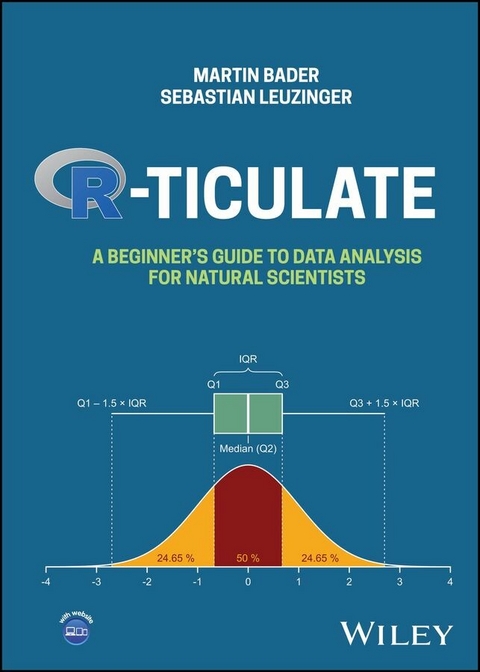
R-ticulate (eBook)
224 Seiten
Wiley (Verlag)
978-1-119-71802-4 (ISBN)
An accessible learning resource that develops data analysis skills for natural science students in an efficient style using the R programming language
R-ticulate: A Beginner's Guide to Data Analysis for Natural Scientists is a compact, example-based, and user-friendly statistics textbook without unnecessary frills, but instead filled with engaging, relatable examples, practical tips, online exercises, resources, and references to extensions, all on a level that follows contemporary curricula taught in large parts of the world.
The content structure is unique in the sense that statistical skills are introduced at the same time as software (programming) skills in R. This is by far the best way of teaching from the authors' experience.
Readers of this introductory text will find:
- Explanations of statistical concepts in simple, easy-to-understand language
- A variety of approaches to problem solving using both base R and tidyverse
- Boxes dedicated to specific topics and margin text that summarizes key points
- A clearly outlined schedule organized into 12 chapters corresponding to the 12 semester weeks of most universities
While at its core a traditional printed book, R-ticulate: A Beginner's Guide to Data Analysis for Natural Scientists comes with a wealth of online teaching material, making it an ideal and efficient reference for students who wish to gain a thorough understanding of the subject, as well as for instructors teaching related courses.
Martin Bader gained an MSc in geography at Saarland University in Germany and an MSc in biology at Waikato University, New Zealand. He earned a PhD in plant ecology at the University of Basel, Switzerland. After post-doctoral stints in Switzerland and Australia he joined the New Zealand Forest Research Institute as a forest ecologist and biostatistician. Following a senior lecturer appointment at Auckland University of Technology, New Zealand, he is now a professor of forest ecology at Linnaeus University, Sweden. He has taught undergraduate and postgraduate courses in statistics at universities and research institutes in various parts of the world. His research focuses on the physiological responses of plants to climate change and their biotic interactions.
Sebastian Leuzinger did his first degree in marine biology at James Cook University, Australia, with a postgraduate degree in statistics (University of Neuchatel, Switzerland) and a PhD in plant ecology (University of Basel, Switzerland). He has done post-doctoral studies at ETH Zurich, Switzerland, in forest ecology and modelling before joining Auckland University of Technology where he is a full professor in ecology. He has taught undergraduate and postgraduate statistics for natural scientists for over a decade. His research is on global change impacts on plants, with a special interest in meta-analysis of global change experiments.
An accessible learning resource that develops data analysis skills for natural science students in an efficient style using the R programming language R-ticulate: A Beginner s Guide to Data Analysis for Natural Scientists is a compact, example-based, and user-friendly statistics textbook without unnecessary frills, but instead filled with engaging, relatable examples, practical tips, online exercises, resources, and references to extensions, all on a level that follows contemporary curricula taught in large parts of the world. The content structure is unique in the sense that statistical skills are introduced at the same time as software (programming) skills in R. This is by far the best way of teaching from the authors experience. Readers of this introductory text will find: Explanations of statistical concepts in simple, easy-to-understand language A variety of approaches to problem solving using both base R and tidyverse Boxes dedicated to specific topics and margin text that summarizes key points A clearly outlined schedule organized into 12 chapters corresponding to the 12 semester weeks of most universities While at its core a traditional printed book, R-ticulate: A Beginner s Guide to Data Analysis for Natural Scientists comes with a wealth of online teaching material, making it an ideal and efficient reference for students who wish to gain a thorough understanding of the subject, as well as for instructors teaching related courses.
1
Hypotheses, Variables, Data
In a world where information circulates at unprecedented speed and almost exclusively via the internet, often on indiscriminate platforms, it has become increasingly difficult to distinguish between fact and fake, between true and false, and between evidence and opinion. One admittedly non‐spectacular, yet indispensable way to confidently plough our way through the jungle of those dichotomies is learning and understanding the basics of statistical thinking. Thinking statistically needs training, as it is not intuitive. Humans are particularly bad at ‘collecting’ data. For example, the perception of whether we had a ‘warm’ or ‘cold’ winter will depend on a wealth of subjective factors such as how much time someone has spent outdoors, and likely shows little correlation with the actual average temperature of that particular winter. Similarly, people perceive risks in life in an utterly ‘non‐statistical’ way. While, statistically, the largest risks for early death in most western countries are sugar intake and lack of exercise, we often perceive the risk of an airplane crashing or a great white shark attack as much more threatening to our lives. In fact, the mentioned risks are four to five orders of magnitude (about 100,000 times) apart!
Human perception is a notoriously bad statistician
In this introductory chapter, we will set the foundations for ‘statistical thinking’, and the most basic statistical skills, which are the pillars that scientific thinking in a broader sense rests on. From our own experience, confusion at a later stage of someone's scientific career is often caused by a lack of knowledge of the fundamentals of statistical principles. For example, we often get approached by students asking us for statistical help, but then the initial conversation shows that the student is not clear about how many variables they are looking at, what their nature is, which of them might be a response or a predictor variable, what the unit of replication is, and so forth. Confusion can also originate following data collection in the absence of a sound scientific hypothesis, or from the absence of a sound study design. Pretty much everything is bound to go wrong from there if these foundations are not laid in time. The purpose of this chapter is therefore to introduce a basic statistical vocabulary, including the formation of a good scientific hypothesis, and how it relates to your data. This also includes training ourselves to dissect and categorise the datasets we encounter. We need to clarify the number of variables we are looking at, as well as their nature and purpose in the dataset.
Alongside all this, we will slowly ease you into the use of the statistical software ‘R’. Despite this adding an element of complexity, it is useful to learn the theory at the same time as the use of a software. We recommend that you replicate our examples on your computer to get a hands‐on experience.
1.1 Occam's Razor
The principle of parsimony (or Occam's razor) is an extremely useful one that should accompany us not only in our statistical thinking, but also generally in all our scientific work. The idea goes back to William of Ockham, a medieval philosopher, who articulated the superiority of a simple as opposed to a more complex explanation for a phenomenon, given equal explanatory power. An illustrative example is the heliocentric model (the earth rotating around the sun) versus the geocentric model (which has the Earth in the centre of the solar system). Both are (or were) used to explain the trajectories of objects in the sky. It turns out that the heliocentric model is far simpler with equal or superior explanatory power, and is thus preferable. The search for the simplest possible explanation has been at the origin of many scientific discoveries, and it is useful to let this principle guide us throughout all stages of planning and conducting our data collection and analysis. The iconic phrase ‘It is in vain to do with more what can be done with fewer’ is applicable to the various stages of scientific research process:
‘It is in vain to do with more what can be done with fewer’
- (1) Planning stage. What is our hypothesis? What data do we need to answer the question? The clearer our (scientific) question is formulated, the easier it is to decide what kind of data we need to collect. ‘De‐cluttering’ the relationship between the question we want to answer and the data we collect can save us an enormous amount of time and frustration.
- (2) Data cleansing and organising stage. Remove any unnecessary element in our data, use minimal (but unique) nomenclature, both for variable names and values. A well organised and simplified dataset forces us to gain a much better understanding of it.
- (3) Analysis stage. Use the minimum number of explanatory variables (and their interactions) that best explains the patterns in your response variables. Every additional explanatory variable will explain some variation in the response by pure chance. We will get to know statistical tools that help us decide on the most parsimonious model, i.e. the smallest set of explanatory variables that explain the most variation in the response variable(s).
- (4) Presentation stage. Once we are ready to convey our (statistical) findings, we again use ‘Occam's razor’ to reduce and ‘distill’ our texts, figures, and tables. This means the removal of any frills that do not serve to make our results more comprehensible. Often, information (for instance, graphs) can be condensed, white space can be minimised or used for insets. In short, we maximise the ratio of information conveyed over the space used (see Chapter 6).
We will revisit most of the aforementioned strategies in chapters to follow. The guiding principle can be extended to many more areas of science not covered in this book, such as scientific writing and oral presentations.
1.2 Scientific Hypotheses
Sometimes we are confronted with complete datasets that we obtain from somewhere, which we then have to analyse. Other times, we pose the scientific question ourselves, and we then set out to collect the data. In both cases, we need to be absolutely clear what question we can or want to answer, as this question is linked with our scientific hypothesis. A scientific hypothesis is a well‐founded assumption that must be testable. For example, ‘The majority of consumers under 20 years of age prefer to pay cashless’, serves as a scientific hypothesis, while ‘Young people prefer to pay by card’ lacks the level of precision required for a scientific hypothesis that we can test, but it may serve as an idea that could lead to a scientific hypothesis. A mismatch between an early (often vague) idea of what we want to research, the resulting hypothesis, and the data we set out to collect, can lead to much confusion.
Be absolutely clear what question you want to answer, and how it could be turned into a hypothesis!
Say, we are interested in biodiversity changes in rock pools on a rocky shore along a tidal gradient. This initial idea could lead to various hypotheses, which would require different data collections. If our hypothesis is ‘The closer the rock pools to the high tide mark, the fewer species per pool’, we would want to count the number of species per rock pool. However, if our hypothesis is ‘species A, B, and C become more abundant moving from the low to the high tide mark, while species D, E, and F become less abundant’, then we would count the number of individuals per species and rock pool. The hypothesis ‘Biodiversity decreases along a tidal gradient’ may not be precise enough to decide exactly what kind of data need to be collected. It is always advisable to have a clear idea of the units we are using (also referred to as the ‘metric’, or the ‘reference metric’ to refer to the denominator of the metric only). For example, if we count the number of species per pool, we will get a fundamentally different outcome compared to if we had counted the number of species per cubic metre of water, or per square metre of rock pool surface. In some instances, the choice of the reference metric can completely change the meaning of the data: while the ‘cases of Covid‐19 per 1000 people’ in a country can increase from one week to another, the ‘cases of Covid‐19 per 1000 administered Covid tests’ can decrease at the same time. These examples illustrate how quickly confusion can arise, which can lead to misinformation, but also how easily a statistically uninformed audience can deliberately be misled. Having a crystal clear idea of what the research question is, what hypothesis we test, and what data we need to collect is therefore pivotal not only for our own work, but also to scrutinise and criticise data or findings that are presented to us.
The aforementioned considerations are important, but so far they are purely theoretical. To really understand and ‘experience’ these issues, we need to ‘leave the classroom’ and get our hands dirty!
What units are my variables in? What reference metrics am I using?
1.3 The Choice of a Software
This topic can be delicate, as people's beliefs, experiences, preferences, and even commercial...
| Erscheint lt. Verlag | 8.7.2024 |
|---|---|
| Sprache | englisch |
| Themenwelt | Mathematik / Informatik ► Mathematik ► Statistik |
| ISBN-10 | 1-119-71802-3 / 1119718023 |
| ISBN-13 | 978-1-119-71802-4 / 9781119718024 |
| Informationen gemäß Produktsicherheitsverordnung (GPSR) | |
| Haben Sie eine Frage zum Produkt? |
Größe: 18,3 MB
Kopierschutz: Adobe-DRM
Adobe-DRM ist ein Kopierschutz, der das eBook vor Mißbrauch schützen soll. Dabei wird das eBook bereits beim Download auf Ihre persönliche Adobe-ID autorisiert. Lesen können Sie das eBook dann nur auf den Geräten, welche ebenfalls auf Ihre Adobe-ID registriert sind.
Details zum Adobe-DRM
Dateiformat: EPUB (Electronic Publication)
EPUB ist ein offener Standard für eBooks und eignet sich besonders zur Darstellung von Belletristik und Sachbüchern. Der Fließtext wird dynamisch an die Display- und Schriftgröße angepasst. Auch für mobile Lesegeräte ist EPUB daher gut geeignet.
Systemvoraussetzungen:
PC/Mac: Mit einem PC oder Mac können Sie dieses eBook lesen. Sie benötigen eine
eReader: Dieses eBook kann mit (fast) allen eBook-Readern gelesen werden. Mit dem amazon-Kindle ist es aber nicht kompatibel.
Smartphone/Tablet: Egal ob Apple oder Android, dieses eBook können Sie lesen. Sie benötigen eine
Geräteliste und zusätzliche Hinweise
Buying eBooks from abroad
For tax law reasons we can sell eBooks just within Germany and Switzerland. Regrettably we cannot fulfill eBook-orders from other countries.
aus dem Bereich


