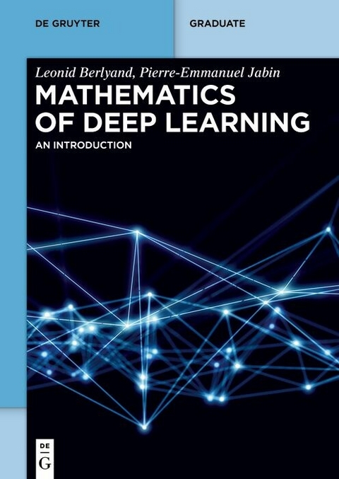
Mathematics of Deep Learning (eBook)

132 Seiten
De Gruyter (Verlag)
978-3-11-102580-3 (ISBN)
The goal of this book is to provide a mathematical perspective on some key elements of the so-called deep neural networks (DNNs). Much of the interest in deep learning has focused on the implementation of DNN-based algorithms. Our hope is that this compact textbook will offer a complementary point of view that emphasizes the underlying mathematical ideas. We believe that a more foundational perspective will help to answer important questions that have only received empirical answers so far.
The material is based on a one-semester course Introduction to Mathematics of Deep Learning' for senior undergraduate mathematics majors and first year graduate students in mathematics. Our goal is to introduce basic concepts from deep learning in a rigorous mathematical fashion, e.g introduce mathematical definitions of deep neural networks (DNNs), loss functions, the backpropagation algorithm, etc. We attempt to identify for each concept the simplest setting that minimizes technicalities but still contains the key mathematics.
Leonid Berland joined the Pennsylvania State University in 1991 where he is currently a Professor of Mathematics and a member of the Materials Research Institute. He is a founding co-director of the Penn State Centers for Interdisciplinary Mathematics and for Mathematics of Living and Mimetic Matter. He is known for his works at the interface between mathematics and other disciplines such as physics, materials sciences, life sciences, and most recently computer science. He has co-authored, Getting Acquainted with Homogenization and Multiscale,Birkhäuser 2018 and Introduction to the Network Approximation Method for Materials Modeling, Cambridge University Press, 2012. His interdisciplinary works received research awards from leading research agencies in the USA, such as NSF, the US Department of Energy, and the National Institute of Health as well as internationally (Bi-National Science Foundation and NATO). Most recently his work was recognized with the Humboldt Research Award of 2021. His teaching excellence was recognized by C.I. Noll Award for Excellence in Teaching by Eberly College of Science at Penn State.
Pierre-Emmanuel Jabin is currently Professor of Mathematics at the Pennsylvania State University since August 2020 previously he was a Professor at the University of Maryland from 2011 to 2020, where he was also director of the Center for Scientific Computation and Mathematical Modeling from 2016 to 2020. Jabin's work in applied mathematics is internationally recognized and he has made seminal contributions to the theory and applications of many-particle/multi-agent systems together with advection and transport phenomena. Jabin was an invited speaker at the International Congress of Mathematicians in Rio de Janeiro in 2018.
4 The fundamentals of artificial neural networks
4.1 Basic definitions
In this book, we focus on deep learning, which is a type of machine learning based on artificial neural networks (ANNs), which involve several layers of so-called neuron functions. This kind of architecture was loosely inspired by the biological neural networks in animals’ brains.
The key building block of ANNs is what we call here a neuron function. A neuron function is a very simplified mathematical representation of a biological neuron dating back to [34]. This naturally leads to various ways of organizing those neuron functions into interacting networks that are capable of complex tasks.
The perceptron, introduced in [43] (see also [35]), is one of the earliest one layer ANNs. Nowadays, multiple layers are typically used instead because neurons in the same layer are not connected, but neurons can interact with neurons in other layers.
We present in this chapter a rather common architecture for classifiers, which is based on so-called feedforward networks, which are networks with no cycles. A “cycle” means that the output of one layer becomes the input of a previous layer. More complex networks can also be used with some cycles between layers (so-called recurrent neural networks; see for example [11], [17]).
Finally as one readily sees, ANNs typically require a very large number of parameters. This makes identifying the best choice for those coefficients delicate and leads to the important question of learning the parameters, which is discussed later in this book.
Definition 4.1.1.
A neuron function f:Rn→R is a mapping of the form (see Fig. 4.1)
where λ:R→R is a continuous non-linear function called the activation function, α∈Rn is a vector of weights, and scalar β∈R is called the bias. Here, α·x is the inner product on Rn.
A typical example of an activation function is ReLU (Rectified Linear Unit), defined as follows (see Fig. 4.2):
ReLU is a very simple non-linear function composed of two linear functions that model the threshold between an “inactive” and an “active” state of the neuron.
Figure 4.1 A neuron function input x∈Rn, vector of weights α=(α1,…,αn), bias β, and output scalar f(x)=λ(α·x+β).
Figure 4.2 ReLU function. β, “bias” constant.
ReLU is a simple way to model a neuron in a brain which has two states: resting (resting potential) and active (firing). Incoming impulses from other neurons can change the state from resting to active, but the impulse needs to reach a certain threshold first. Thus, ReLU’s change from constant 0 to a linear function at xthresh=β reflects the change from resting to active at this threshold.
Figure 4.3 Layer of neurons fI, 1≤i≤4, with vector of input data xj. Weights αij are assigned to each edge connecting xj and fi, n=3, m=4.
Since the output of a neuron function is a single number, we can combine several neurons to create a vector-valued function called a layer function.
Definition 4.1.2.
A layer function g:Rn→Rm is a mapping of the form
where each fi:Rn→R is a neuron function of the form (4.1) with its own vector of parameters αi=(αi1,…,αin) and biases βi, i=1,…,m.
Remark 4.1.2.
When discussing layers, it is important to distinguish between the layer nodes and the layer function that connects them. There are two columns of nodes in Fig. 4.3, which are commonly referred to as two layers. However, according to Definition 4.1.2, Fig. 4.3 depicts a single layer function. Thus, it is important to distinguish between columns of nodes in diagrammatic representations of layers as in Fig. 4.3 and the layer function that connects them defined in (4.3). This is illustrated in Fig. 4.3, where the nodes x=(x1,x2,x3) can be referred to as the nodes of the input vector and the output vector of the layer function is given by (4.3). In such a situation, one may commonly refer to two layers of nodes: the input layer composed of the nodes corresponding to the coordinates xi of x and the output layer composed of the m nodes corresponding to the coordinates yi of y=g(x). For a general multilayer network defined in Definition 4.1.3, if we consider M layer functions, we will have M+1 layers of nodes. We simply write layer for layer of nodes, and often refer to individual nodes within a layer as neurons (vs. the layer functions or neuron functions connecting those).
Thus, the layer function is determined by a matrix of parameters,
and a vector of biases,
Hence, (4.3) may be written
where λ¯:Rm→Rm is the vectorial activation function defined as
for a scalar activation function λ as in Definition 4.1.1.
See Fig. 4.3 for a diagram of a layer function. This figure shows a layer as a graph with two columns of nodes. The right column depicts neuron functions in the layer, while the left column depicts three real numbers (data) which are input to the layer. The edge connecting the ith input with the jth neuron is multiplied by the parameter value αij from the matrix of parameters.
Definition 4.1.3.
An artificial neural network (ANN) is a function h:Rn→Rm of the form
where each hi:Rni−1→Rni is a layer function (see Definition 4.1.2) with its own matrix of parameters Ai and its own vector of biases βi.
Fig. 4.4 shows an ANN composed of two layers. The layer function in Fig. 4.4 between input and output is called a hidden layer (hidden from the user) because its output is passed to another layer, not directly to the user. The number of neurons ni in the ith layer is called the layer’s width, while the total number M of layers in an ANN is the depth of the ANN. The numbers n1,…,nM and M comprise the architecture of this network. ANNs with more than one layer are referred to as deep neural networks (DNNs).
Figure 4.4 Simple network with input layer and two layer functions, n=n0=4, n1=6, m=n2=3.
This network is called fully connected because for all but the last layer, each neuron provides input to each neuron in the next layer. That is, each node in each column of the graph in Fig. 4.4 is connected to each node in the...
| Erscheint lt. Verlag | 27.4.2023 |
|---|---|
| Reihe/Serie | De Gruyter Textbook | De Gruyter Textbook |
| Zusatzinfo | 20 b/w and 30 col. ill. |
| Sprache | englisch |
| Themenwelt | Mathematik / Informatik ► Informatik ► Programmiersprachen / -werkzeuge |
| Mathematik / Informatik ► Mathematik | |
| Schlagworte | artificial neural networks (ANNs) • Deep learning • Deep Neural Networks (DNNs) • Faltungsneuronale Netze • Künstliche Neuronale Netze • Künstliche neuronale Netzwerke • machine learning • Machine Learning, Deep Learning, Artificial Neural Networks (ANNs), Regression, Deep Neural Networks (DNNs), • Maschinelles Lernen • Regression • Tiefe Neuronale Netzwerke • Tiefes Lernen |
| ISBN-10 | 3-11-102580-2 / 3111025802 |
| ISBN-13 | 978-3-11-102580-3 / 9783111025803 |
| Informationen gemäß Produktsicherheitsverordnung (GPSR) | |
| Haben Sie eine Frage zum Produkt? |
Größe: 11,7 MB
DRM: Digitales Wasserzeichen
Dieses eBook enthält ein digitales Wasserzeichen und ist damit für Sie personalisiert. Bei einer missbräuchlichen Weitergabe des eBooks an Dritte ist eine Rückverfolgung an die Quelle möglich.
Dateiformat: EPUB (Electronic Publication)
EPUB ist ein offener Standard für eBooks und eignet sich besonders zur Darstellung von Belletristik und Sachbüchern. Der Fließtext wird dynamisch an die Display- und Schriftgröße angepasst. Auch für mobile Lesegeräte ist EPUB daher gut geeignet.
Systemvoraussetzungen:
PC/Mac: Mit einem PC oder Mac können Sie dieses eBook lesen. Sie benötigen dafür die kostenlose Software Adobe Digital Editions.
eReader: Dieses eBook kann mit (fast) allen eBook-Readern gelesen werden. Mit dem amazon-Kindle ist es aber nicht kompatibel.
Smartphone/Tablet: Egal ob Apple oder Android, dieses eBook können Sie lesen. Sie benötigen dafür eine kostenlose App.
Geräteliste und zusätzliche Hinweise
Buying eBooks from abroad
For tax law reasons we can sell eBooks just within Germany and Switzerland. Regrettably we cannot fulfill eBook-orders from other countries.
aus dem Bereich


