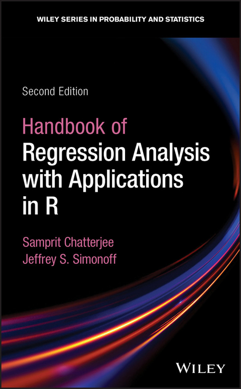
Handbook of Regression Analysis With Applications in R (eBook)
384 Seiten
Wiley (Verlag)
978-1-119-39248-4 (ISBN)
Handbook and reference guide for students and practitioners of statistical regression-based analyses in R
Handbook of Regression Analysis with Applications in R, Second Edition is a comprehensive and up-to-date guide to conducting complex regressions in the R statistical programming language. The authors' thorough treatment of 'classical' regression analysis in the first edition is complemented here by their discussion of more advanced topics including time-to-event survival data and longitudinal and clustered data.
The book further pays particular attention to methods that have become prominent in the last few decades as increasingly large data sets have made new techniques and applications possible. These include:
- Regularization methods
- Smoothing methods
- Tree-based methods
In the new edition of the Handbook, the data analyst's toolkit is explored and expanded. Examples are drawn from a wide variety of real-life applications and data sets. All the utilized R code and data are available via an author-maintained website.
Of interest to undergraduate and graduate students taking courses in statistics and regression, the Handbook of Regression Analysis will also be invaluable to practicing data scientists and statisticians.
Samprit Chatterjee, PhD, is Professor Emeritus of Statistics at New York University. A Fellow of the American Statistical Association, Dr. Chatterjee has been a Fulbright scholar in both Kazakhstan and Mongolia. He is the coauthor of multiple editions of Regression Analysis By Example, Sensitivity Analysis in Linear Regression, A Casebook for a First Course in Statistics and Data Analysis, and the first edition of Handbook of Regression Analysis, all published by Wiley.
Jeffrey S. Simonoff, PhD, is Professor of Statistics at the Leonard N. Stern School of Business of New York University. He is a Fellow of the American Statistical Association, a Fellow of the Institute of Mathematical Statistics, and an Elected Member of the International Statistical Institute. He has authored, coauthored, or coedited more than one hundred articles and seven books on the theory and applications of statistics.
Handbook and reference guide for students and practitioners of statistical regression-based analyses in R Handbook of Regression Analysis with Applications in R, Second Edition is a comprehensive and up-to-date guide to conducting complex regressions in the R statistical programming language. The authors' thorough treatment of "e;classical"e; regression analysis in the first edition is complemented here by their discussion of more advanced topics including time-to-event survival data and longitudinal and clustered data. The book further pays particular attention to methods that have become prominent in the last few decades as increasingly large data sets have made new techniques and applications possible. These include: Regularization methods Smoothing methods Tree-based methods In the new edition of the Handbook, the data analyst's toolkit is explored and expanded. Examples are drawn from a wide variety of real-life applications and data sets. All the utilized R code and data are available via an author-maintained website. Of interest to undergraduate and graduate students taking courses in statistics and regression, the Handbook of Regression Analysis will also be invaluable to practicing data scientists and statisticians.
Samprit Chatterjee, PhD, is Professor Emeritus of Statistics at New York University. A Fellow of the American Statistical Association, Dr. Chatterjee has been a Fulbright scholar in both Kazakhstan and Mongolia. He is the coauthor of multiple editions of Regression Analysis By Example, Sensitivity Analysis in Linear Regression, A Casebook for a First Course in Statistics and Data Analysis, and the first edition of Handbook of Regression Analysis, all published by Wiley. Jeffrey S. Simonoff, PhD, is Professor of Statistics at the Leonard N. Stern School of Business of New York University. He is a Fellow of the American Statistical Association, a Fellow of the Institute of Mathematical Statistics, and an Elected Member of the International Statistical Institute. He has authored, coauthored, or coedited more than one hundred articles and seven books on the theory and applications of statistics.
CHAPTER ONE
Multiple Linear Regression
- 1.1 Introduction
- 1.2 Concepts and Background Material
- 1.3 Methodology
- 1.4 Example—Estimating Home Prices
- 1.5 Summary
1.1 Introduction
This is a book about regression modeling, but when we refer to regression models, what do we mean? The regression framework can be characterized in the following way:
- We have one particular variable that we are interested in understanding or modeling, such as sales of a particular product, sale price of a home, or voting preference of a particular voter. This variable is called the target, response, or dependent variable, and is usually represented by .
- We have a set of other variables that we think might be useful in predicting or modeling the target variable (the price of the product, the competitor's price, and so on; or the lot size, number of bedrooms, number of bathrooms of the home, and so on; or the gender, age, income, party membership of the voter, and so on). These are called the predicting, or independent variables, and are usually represented by , , etc.
Typically, a regression analysis is used for one (or more) of three purposes:
- modeling the relationship between and ;
- prediction of the target variable (forecasting);
- and testing of hypotheses.
In this chapter, we introduce the basic multiple linear regression model, and discuss how this model can be used for these three purposes. Specifically, we discuss the interpretations of the estimates of different regression parameters, the assumptions underlying the model, measures of the strength of the relationship between the target and predictor variables, the construction of tests of hypotheses and intervals related to regression parameters, and the checking of assumptions using diagnostic plots.
1.2 Concepts and Background Material
1.2.1 THE LINEAR REGRESSION MODEL
The data consist of observations, which are sets of observed values that represent a random sample from a larger population. It is assumed that these observations satisfy a linear relationship,
where the coefficients are unknown parameters, and the are random error terms. By a linear model, it is meant that the model is linear in the parameters; a quadratic model,
paradoxically enough, is a linear model, since and are just versions of and .
It is important to recognize that this, or any statistical model, is not viewed as a true representation of reality; rather, the goal is that the model be a useful representation of reality. A model can be used to explore the relationships between variables and make accurate forecasts based on those relationships even if it is not the “truth.” Further, any statistical model is only temporary, representing a provisional version of views about the random process being studied. Models can, and should, change, based on analysis using the current model, selection among several candidate models, the acquisition of new data, new understanding of the underlying random process, and so on. Further, it is often the case that there are several different models that are reasonable representations of reality. Having said this, we will sometimes refer to the “true” model, but this should be understood as referring to the underlying form of the currently hypothesized representation of the regression relationship.
FIGURE 1.1: The simple linear regression model. The solid line corresponds to the true regression line, and the dotted lines correspond to the random errors .
The special case of (1.1) with corresponds to the simple regression model, and is consistent with the representation in Figure 1.1. The solid line is the true regression line, the expected value of given the value of . The dotted lines are the random errors that account for the lack of a perfect association between the predictor and the target variables.
1.2.2 ESTIMATION USING LEAST SQUARES
The true regression function represents the expected relationship between the target and the predictor variables, which is unknown. A primary goal of a regression analysis is to estimate this relationship, or equivalently, to estimate the unknown parameters . This requires a data‐based rule, or criterion, that will give a reasonable estimate. The standard approach is least squares regression, where the estimates are chosen to minimize
Figure 1.2 gives a graphical representation of least squares that is based on Figure 1.1. Now the true regression line is represented by the gray line, and the solid black line is the estimated regression line, designed to estimate the (unknown) gray line as closely as possible. For any choice of estimated parameters , the estimated expected response value given the observed predictor values equals
FIGURE 1.2: Least squares estimation for the simple linear regression model, using the same data as in Figure 1.1. The gray line corresponds to the true regression line, the solid black line corresponds to the fitted least squares line (designed to estimate the gray line), and the lengths of the dotted lines correspond to the residuals. The sum of squared values of the lengths of the dotted lines is minimized by the solid black line.
and is called the fitted value. The difference between the observed value and the fitted value is called the residual, the set of which is represented by the signed lengths of the dotted lines in Figure 1.2. The least squares regression line minimizes the sum of squares of the lengths of the dotted lines; that is, the ordinary least squares (OLS) estimates minimize the sum of squares of the residuals.
In higher dimensions (), the true and estimated regression relationships correspond to planes () or hyperplanes (), but otherwise the principles are the same. Figure 1.3 illustrates the case with two predictors. The length of each vertical line corresponds to a residual (solid lines refer to positive residuals, while dashed lines refer to negative residuals), and the (least squares) plane that goes through the observations is chosen to minimize the sum of squares of the residuals.
FIGURE 1.3: Least squares estimation for the multiple linear regression model with two predictors. The plane corresponds to the fitted least squares relationship, and the lengths of the vertical lines correspond to the residuals. The sum of squared values of the lengths of the vertical lines is minimized by the plane.
The linear regression model can be written compactly using matrix notation. Define the following matrix and vectors as follows:
The regression model (1.1) is then
The normal equations [which determine the minimizer of 1.2] can be shown (using multivariate calculus) to be
which implies that the least squares estimates satisfy
The fitted values are then
where is the so‐called “hat” matrix (since it takes to ). The residuals thus satisfy
or
1.2.3 ASSUMPTIONS
The least squares criterion will not necessarily yield sensible results unless certain assumptions hold. One is given in (1.1) — the linear model should be appropriate. In addition, the following assumptions are needed to justify using least squares regression.
- The expected value of the errors is zero ( for all ). That is, it cannot be true that for certain observations the model is systematically too low, while for others it is systematically too high. A violation of this assumption will lead to difficulties in estimating . More importantly, this reflects that the model does not include a necessary systematic component, which has instead been absorbed into the error terms.
- The variance of the errors is constant ( for all ). That is, it cannot be true that the strength of the model is greater for some parts of the population (smaller ) and less for other parts (larger ). This assumption of constant variance is called homoscedasticity, and its violation (nonconstant variance) is called heteroscedasticity. A violation of this assumption means that the least squares estimates are not as efficient as they could be in estimating the true parameters, and better estimates are available. More importantly, it also results in poorly calibrated confidence and (especially) prediction intervals.
- The errors are uncorrelated with each other. That is, it cannot be true that knowing that the...
| Erscheint lt. Verlag | 30.7.2020 |
|---|---|
| Reihe/Serie | Wiley Series in Probability and Statistics |
| Sprache | englisch |
| Themenwelt | Mathematik / Informatik ► Mathematik ► Statistik |
| Mathematik / Informatik ► Mathematik ► Wahrscheinlichkeit / Kombinatorik | |
| Schlagworte | Data Analysis • Datenanalyse • Regression Analysis • Regressionsanalyse • R (Programm) • Statistical Software / R • Statistics • Statistik • Statistiksoftware / R |
| ISBN-10 | 1-119-39248-9 / 1119392489 |
| ISBN-13 | 978-1-119-39248-4 / 9781119392484 |
| Haben Sie eine Frage zum Produkt? |
Größe: 17,5 MB
Kopierschutz: Adobe-DRM
Adobe-DRM ist ein Kopierschutz, der das eBook vor Mißbrauch schützen soll. Dabei wird das eBook bereits beim Download auf Ihre persönliche Adobe-ID autorisiert. Lesen können Sie das eBook dann nur auf den Geräten, welche ebenfalls auf Ihre Adobe-ID registriert sind.
Details zum Adobe-DRM
Dateiformat: EPUB (Electronic Publication)
EPUB ist ein offener Standard für eBooks und eignet sich besonders zur Darstellung von Belletristik und Sachbüchern. Der Fließtext wird dynamisch an die Display- und Schriftgröße angepasst. Auch für mobile Lesegeräte ist EPUB daher gut geeignet.
Systemvoraussetzungen:
PC/Mac: Mit einem PC oder Mac können Sie dieses eBook lesen. Sie benötigen eine
eReader: Dieses eBook kann mit (fast) allen eBook-Readern gelesen werden. Mit dem amazon-Kindle ist es aber nicht kompatibel.
Smartphone/Tablet: Egal ob Apple oder Android, dieses eBook können Sie lesen. Sie benötigen eine
Geräteliste und zusätzliche Hinweise
Buying eBooks from abroad
For tax law reasons we can sell eBooks just within Germany and Switzerland. Regrettably we cannot fulfill eBook-orders from other countries.
aus dem Bereich


