Statistics for Chemical and Process Engineers (eBook)
XXVI, 414 Seiten
Springer International Publishing (Verlag)
978-3-319-21509-9 (ISBN)
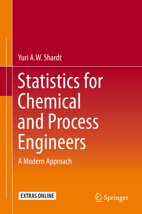
A coherent, concise and comprehensive course in the statistics needed for a modern career in chemical engineering; covers all of the concepts required for the American Fundamentals of Engineering examination.
This book shows the reader how to develop and test models, design experiments and analyse data in ways easily applicable through readily available software tools like MS Excel® and MATLAB®. Generalized methods that can be applied irrespective of the tool at hand are a key feature of the text.
The reader is given a detailed framework for statistical procedures covering:
· data visualization;
· probability;
· linear and nonlinear regression;
· experimental design (including factorial and fractional factorial designs); and
· dynamic process identification.
Main concepts are illustrated with chemical- and process-engineering-relevant examples that can also serve as the bases for checking any subsequent real implementations. Questions are provided (with solutions available for instructors) to confirm the correct use of numerical techniques, and templates for use in MS Excel and MATLAB can also be downloaded from extras.springer.com.
With its integrative approach to system identification, regression and statistical theory, Statistics for Chemical and Process Engineers provides an excellent means of revision and self-study for chemical and process engineers working in experimental analysis and design in petrochemicals, ceramics, oil and gas, automotive and similar industries and invaluable instruction to advanced undergraduate and graduate students looking to begin a career in the process industries.
Dr. Yuri A.W. Shardt is currently an Alexander von Humboldt Fellow working at the University of Duisberg-Essen in fault detection and isolation for complex systems. He has written many papers appearing in journals such as Automatica, Journal of Process Control, and Industrial and Engineering Chemistry Research on topics ranging from systems identification, soft sensor development, and process control, as well as attending and presenting his research at numerous conferences. He has taught various courses in the intersection between statistics, chemical engineering, process control, EXCEL, and MATLAB®. Dr. Shardt completed his doctoral degree under the supervision of Professor Biao Huang at the University of Alberta. His thesis examined the methods for extracting valuable data for system identification from data historians for application to soft sensor design. In addition to his academic work, he has spent considerable time in industry working on implementing various process control solutions.
Prof. Dr. Yuri A. W. Shardt is currently the chair of the Department of Automation Engineering (DE: Fachgebiet Automatisierungstechnik) in the Faculty of Computer Science and Automation (DE: Fakultät Informatik und Automatisierung) at the Technical University of Ilmenau (DE: Technische Universität Ilmenau), working in the fields of big data, including process identification and monitoring with an emphasis on the development and industrial implementation of soft sensors; holistic control, including the development of advanced control strategies for complex industrial process; and the smart world, including such implementations as smart factories, smart home, Industry 4.0, and smart grids. Previously, he worked at the University of Waterloo in the Department of Chemical Engineering and at the University of Duisburg-Essen in the Institute of Control and Complex Systems (DE: Fachgebiet Automatisierungstechnik und komplexe Systeme, AKS) as an Alexander von Humboldt Fellow. He has written 30 papers appearing in such journals as Automatica, Journal of Process Control, IEEE Transactions on Industrial Electronics, and Industrial and Engineering Chemistry Research on topics ranging from system identification, soft sensor development, to process control. He has presented his research at numerous conferences and taught various courses in the intersection between statistics, chemical engineering, process control, EXCEL®, and MATLAB®. Prof. Dr. Shardt completed his doctoral degree under the supervision of Prof. Dr. Biao Huang at the University of Alberta. His thesis examined the methods for extracting valuable data for system identification from data historians for application to soft sensor design. In addition to his academic work, he has spent considerable time in industry working on implementing various process control solutions. He also has interests in linguistics, as well as software internationalisation and localisation.
Foreword 6
Contents 10
List of Figures 18
List of Tables 24
Chapter 1: Introduction to Statistics and Data Visualisation 28
1.1 Basic Descriptive Statistics 30
1.1.1 Measures of Central Tendency 30
1.1.2 Measures of Dispersion 31
1.1.3 Other Statistical Measures 33
1.1.3.1 Quantiles 33
1.1.3.2 Outliers 35
1.2 Data Visualisation 35
1.2.1 Bar Charts and Histograms 36
1.2.2 Pie Charts 37
1.2.3 Line Charts 37
1.2.4 Box-and-Whisker Plots 39
1.2.5 Scatter Plots 40
1.2.6 Probability Plots 40
1.2.7 Tables 45
1.2.8 Sparkplots 46
1.2.9 Other Data Visualisation Methods 46
1.3 Friction Factor Example 48
1.3.1 Explanation of the Data Set 48
1.3.2 Summary Statistics 50
1.3.3 Data Visualisation 51
1.3.4 Some Observations on the Data Set 53
1.4 Further Reading 54
1.5 Chapter Problems 55
1.5.1 Basic Concepts 55
1.5.2 Short Exercises 56
1.5.3 Computational Exercises 56
Chapter 2: Theoretical Foundation for Statistical Analysis 58
2.1 Statistical Axioms and Definitions 58
Example 2.1: Determining the Probability Space 59
Example 2.2: Determining Acceptable Probability Density Functions 61
Example 2.3: Computing Mean and Variance from the Probability Density Function 63
2.2 Expectation Operator 64
Example 2.4: Using the Expectation Operator 64
2.3 Multivariate Statistics 65
Example 2.5: Dealing with a Multivariate Distribution 67
2.4 Common Statistical Distributions 70
2.4.1 Normal Distribution 70
2.4.2 Student´s t-Distribution 72
2.4.3 chi2-Distribution 73
2.4.4 F-Distribution 74
2.4.5 Binomial Distribution 75
2.4.6 Poisson Distribution 77
2.5 Parameter Estimation 77
2.5.1 Considerations for Parameter Estimation 78
2.5.2 Methods of Parameter Estimation 79
2.5.2.1 Method of Moments 79
Example 2.6: Method of Moments for a Normal Distribution 80
2.5.2.2 Maximum Likelihood Method 81
Example 2.7: Maximum Likelihood Estimates for a Normal Distribution 82
2.5.3 Remarks on Estimating the Mean, Variance, and Standard Deviation 84
2.6 Central Limit Theorem 85
2.7 Hypothesis Testing and Confidence Intervals 85
2.7.1 Computing the Critical Value 88
2.7.2 Converting Confidence Intervals 89
2.7.3 Testing the Mean 91
Example 2.8: Testing the Mean-Computing a Confidence Interval 91
Example 2.9: Testing the Mean-Hypothesis Testing 92
Example 2.10: Testing the Mean-Unknown Variances 92
Example 2.11: Testing the Mean-Detailed Example 93
2.7.4 Testing the Variance 94
Example 2.12: Testing the Variance 94
2.7.5 Testing a Ratio or Proportion 95
Example 2.13: Testing a Ratio 95
2.7.6 Testing Two Samples 96
2.7.6.1 Testing the Mean 96
Example 2.14: Testing Differences in Means-Variances Known 99
Example 2.15: Testing the Difference in Means-Unknown, Common Mean 100
Example 2.16: Testing Two Means-Unknown Variance 101
Example 2.17: Testing a Paired Mean 102
2.7.6.2 Testing Two Variances 103
Example 2.18: Testing Two Sample Variances 104
2.7.6.3 Testing Two Proportions 104
Example 2.19: Testing Two Proportions 105
2.8 Further Reading 106
2.9 Chapter Problems 106
2.9.1 Basic Concepts 106
2.9.2 Short Exercises 107
2.9.3 Computational Exercises 110
Appendix A2: A Brief Review of Set Theory and Notation 111
Chapter 3: Regression 113
3.1 Regression Analysis Framework 113
3.2 Regression Models 114
3.2.1 Linear and Nonlinear Regression Functions 116
Example 3.1: Linearising Nonlinear Models 116
3.3 Linear Regression 119
3.3.1 Ordinary, Least-Squares Regression 119
3.3.2 Analysis of Variance of the Regression Model 125
3.3.3 Useful Formulae for Ordinary, Least-Squares Regression 128
3.3.4 Computational Example Part I: Determining the Model Parameters 130
3.3.5 Model Validation 133
3.3.5.1 Residual Testing 134
3.3.5.2 Testing for Model Adequacy 136
3.3.5.3 Taking Corrective Action 138
3.3.6 Computational Example Part II: Model Validation 140
3.3.7 Weighted, Least-Squares Regression 142
3.3.7.1 Determining the Weights 144
Example 3.2: Determining the Weights for Weighted, Least-Squares Regression 145
3.4 Nonlinear Regression 146
3.4.1 Gauss-Newton Solution for Nonlinear Regression 147
3.4.2 Useful Formulae for Nonlinear Regression 148
3.4.3 Computational Example of Nonlinear Regression 149
3.5 Models and Their Use 152
3.6 Summative Regression Example 152
3.6.1 Data and Problem Statement 153
3.6.2 Solution 153
3.6.2.1 Simple Linear Model 153
3.6.2.2 Quadratic Model 155
3.6.2.3 Mean Response Intervals 156
3.7 Further Reading 157
3.8 Chapter Problems 157
3.8.1 Basic Concepts 157
3.8.2 Short Exercises 158
3.8.3 Computational Exercises 160
Appendix A3: Nonmatrix Solutions to the Linear, Least-Squares Regression Problem 163
A.1 Nonmatrix Solution for the Ordinary, Least-Squares Case 163
A.2 Nonmatrix Solution for the Weighted, Least-Squares Case 165
Chapter 4: Design of Experiments 167
4.1 Fundamentals of Design of Experiments 167
4.1.1 Sensitivity 168
4.1.2 Confounding and Correlation Between Parameters 168
4.1.3 Blocking 169
4.1.3.1 Rabbit Weight Experiment 169
4.1.3.2 Shoe Wear Example 170
4.1.4 Randomisation 171
4.2 Types of Models 171
4.2.1 Model Use 171
4.3 Framework for the Analysis of Experiments 172
4.4 Factorial Design 173
4.4.1 Factorial Design Models 173
Example 4.1: Full Factorial Design 175
4.4.2 Factorial Analysis 176
4.4.3 Selecting Influential Parameters (Effects) 178
4.4.4 Projection 178
Example 4.2: Analysis of a Full Factorial Experiment 180
4.5 Fractional Factorial Design 183
4.5.1 Notation for Fractional Factorial Experiments 184
4.5.2 Resolution of Fractional Factorial Experiments 184
4.5.3 Confounding in Fractional Factorial Experiments 184
4.5.3.1 Background Information 185
Example 4.3: Modular Arithmetic 185
4.5.3.2 Generators for Fractional Factorial Experiments 186
Example 4.4: Generators and Defining Relationships for a Fractional Factorial Design 186
4.5.3.3 Complete Defining Relationship for Fractional Factorial Experiments 187
4.5.3.4 Complete Confounding Pattern for Fractional Factorial Experiments 187
Example 4.5: Complete Defining Relationship and Confounding Pattern for a Half-Fractional Factorial Example 187
Example 4.6: Confounding Pattern for a Quarter-Fractional Factorial Example 189
4.5.3.5 Higher-Level Designs 190
Example 4.7: Complete Confounding Pattern for a 3-Level Experiment 191
4.5.4 Design Procedure for Fractional Factorial Experiments 192
Example 4.8: Analysing the Structure of a Fractional Factorial Experiment 192
4.5.5 Analysis of Fractional Factorial Experiments 194
4.5.6 Framework for the Analysis of Factorial Designs 195
Example 4.9: Detailed Analysis of a Fractional Factorial Experiment 196
4.6 Blocking and Factorial Design 202
Example 4.10: Blocking and Full Factorial Design 202
Example 4.11: Blocking and Fractional Factorial Design 203
4.7 Generalised Factorial Design 204
4.7.1 Obtaining an Orthogonal Basis 205
4.7.2 Orthogonal Bases for Different Levels 206
4.7.2.1 Case l=2 206
4.7.2.2 Case l=3 207
Example 4.12: Orthogonal Basis for a Mixed-Level Factorial Experiment 208
4.7.2.3 Case l=4 210
4.7.2.4 Generalised Orthonormal Basis Functions for First- and Second-Order Terms 212
4.7.3 Sum of Squares in Generalised Factorial Designs 212
4.7.4 Detailed Mixed-Level Example 213
4.7.4.1 Analysis 214
4.7.4.2 Preprocessing the Data 214
4.7.4.3 Determining the General Model Form 214
4.7.4.4 Obtaining a Basis 215
4.7.4.5 Defining the Linear Regression Problem 215
4.7.4.6 Determining the Model 216
4.7.4.7 Analysing the Residuals 217
4.8 2k Factorial Designs with Centre Point Replicates 218
4.8.1 Orthogonal Basis for 2k Factorial Designs with Centre Point Replicates 219
4.8.2 Factorial Design with Centre Point Example 221
4.8.2.1 Determining the General Model 221
4.8.2.2 Selecting the Orthogonal Basis 222
4.8.2.3 Defining the Linear Regression Problem 222
4.8.2.4 Determining the Model 223
4.8.2.5 Analysing the Residuals 223
4.9 Response Surface Design 224
4.9.1 Central Composite Design 225
4.9.1.1 Determining the Value of ? 226
4.9.2 Optimal Design 227
4.9.3 Response Surface Procedure 227
4.10 Further Reading 228
4.11 Chapter Problems 228
4.11.1 Basic Concepts 228
4.11.2 Short Exercises 229
4.11.3 Computational Exercises 231
Appendix A4: Nonmatrix Approach to the Analysis of 2k-Factorial Design Experiments 234
Chapter 5: Modelling Stochastic Processes with Time Series Analysis 236
5.1 Fundamentals of Time Series Analysis 237
5.1.1 Estimating the Autocovariance and Cross-Covariance and Correlation Functions 240
5.1.2 Obtaining a Stationary Time Series 241
5.1.3 Edmonton Weather Data Series Example 241
5.2 Common Time Series Models 244
5.3 Theoretical Examination of Time Series Models 247
5.3.1 Properties of a White Noise Process 248
5.3.2 Properties of a Moving-Average Process 248
Example 5.1: Example of a Moving-Average Process 250
Example 5.2: Simulation of a Moving-Average Process 252
5.3.3 Properties of an Autoregressive Process 253
Example 5.3: Example of an Autoregressive Process 256
Example 5.4: Simulation of an Autoregressive Process 257
5.3.4 Properties of an Integrating Process 258
Example 5.5: Simulation of an Integrating Process 258
5.3.5 Properties of ARMA and ARIMA Processes 260
Example 5.6: Simulation of an ARMA Process 261
5.3.6 Properties of the Seasonal Component of a Time Series Model 262
Example 5.7: Simulation of the Seasonal Component 263
5.3.7 Summary of the Theoretical Properties for Different Time Series Models 264
5.4 Time Series Modelling 265
5.4.1 Estimating the Time Series Model Parameters 266
5.4.1.1 Yule-Walker Equations for Estimating an Autoregressive Model 266
Example 5.8: Fitting an AR(2) Process Using the Yule-Walker Equations 268
5.4.1.2 Computing the Partial Autocorrelation Function 269
Example 5.9: Partial Autocorrelation for an AR(1) Process 270
5.4.2 Maximum-Likelihood Parameter Estimates for ARMA Models 270
Example 5.10: Exact Solution of the Maximum-Likelihood Equation for an Autoregressive Model 272
Example 5.11: Modelling the Mean Summer Temperature in Edmonton 274
5.4.3 Model Validation for Time Series Models 275
Example 5.12: Validating the Initial Mean Summer Temperature in Edmonton Model 277
5.4.4 Model Prediction and Forecasting Using Time Series Models 278
Example 5.13: Forecasting A Ma(3) Process 281
5.4.4.1 Durbin-Levinson Algorithm 282
Example 5.14: Using the Durbin-Levinson Algorithm to Obtain the Predictor 282
5.5 Frequency-Domain Analysis of Time Series 284
5.5.1 Fourier Transform 284
5.5.2 Periodogram and Its Use in Frequency-Domain Analysis of Time Series 287
Example 5.15: Periodograms for the Edmonton Temperature Series 289
5.6 State-Space Modelling of Time Series 291
5.6.1 State-Space Model for Time Series 291
5.6.2 The Kalman Equation 292
5.6.3 Maximum-Likelihood State-Space Estimates 295
5.7 Comprehensive Example of Time Series Modelling 296
5.7.1 Summary of Available Information 296
5.7.2 Obtaining the Final Univariate Model 297
5.8 Further Reading 298
5.9 Chapter Problems 299
5.9.1 Basic Concepts 300
5.9.2 Short Exercises 301
5.9.3 Computational Exercises 301
Appendix A5: Data Sets for This Chapter 302
A5.1: Edmonton Weather Data Series (1882-2002) 302
A5.2: AR(2) Process Data 306
A5.3: MA(3) Process Data 307
Chapter 6: Modelling Dynamic Processes Using System Identification Methods 308
6.1 Control and Process System Identification 309
6.1.1 Predictability of Process Models 312
6.2 Framework for System Identification 316
6.3 Open-Loop Process Identification 317
6.3.1 Parameter Estimation in Process Identification 317
6.3.2 Model Validation in Process Identification 321
6.3.3 Design of Experiments in Process Identification 323
6.3.4 Final Considerations in Open-Loop Process Identification 325
6.3.4.1 Time Delay 325
6.3.4.2 Drifting and Disturbances 327
6.3.4.3 Linearity 327
6.3.4.4 Time Invariance 328
6.4 Closed-Loop Process Identification 328
6.4.1 Indirect Identification of a Closed-Loop Process 330
6.4.2 Direct Identification of a Closed-Loop Process 331
6.4.3 Joint Input-Output Identification of a Closed-Loop Process 333
6.5 Nonlinear Process Identification 334
6.5.1 Transformation of Nonlinear Models: Wiener-Hammerstein Models 335
6.6 Modelling the Water Level in a Tank 335
6.6.1 Design of Experiment 336
6.6.1.1 Preliminary Identification 337
6.6.1.2 Final Identification 337
6.6.2 Raw Data 338
6.6.3 Linear Model Creation and Validation 339
6.6.3.1 Time Delay Estimation 339
6.6.3.2 Initial Model 340
6.6.3.3 Final Model 341
6.6.4 Nonlinear Model Creation and Validation 343
6.6.5 Final Comments 345
6.7 Further Reading 346
6.8 Chapter Problems 346
6.8.1 Basic Concepts 347
6.8.2 Short Exercises 347
6.8.3 Computational Exercises 349
Appendix A6: Data Sets for This Chapter 349
A6.1: Water Level in Tanks 1 and 2 Data 349
Chapter 7: Using MATLAB for Statistical Analysis 362
7.1 Basic Statistical Functions 362
7.2 Basic Functions for Creating Graphs 362
7.3 The Statistics and Machine Learning Toolbox 366
7.3.1 Probability Distributions 366
7.3.2 Advanced Statistical Functions 366
7.3.3 Useful Probability Functions 367
7.3.4 Linear Regression Analysis 367
7.3.5 Design of Experiments 367
7.4 The System Identification Toolbox 369
7.5 The Econometrics Toolbox 371
7.6 The Signal Processing Toolbox 371
7.7 MATLAB Recipes 372
7.7.1 Periodogram 375
7.7.2 Autocorrelation Plot 376
7.7.3 Correlation Plot 377
7.7.4 Cross-Correlation Plot 377
7.8 MATLAB Examples 379
7.8.1 Linear Regression Example in MATLAB 379
7.8.1.1 Problem Statement for Linear Regression Example 379
7.8.1.2 Solution for Linear Regression Example 379
7.8.2 Nonlinear Regression Example in MATLAB 383
7.8.2.1 Problem Statement for Nonlinear Regression Example 383
7.8.2.2 Problem Solution for Nonlinear Regression Example 383
7.8.3 System Identification Example in MATLAB 386
7.9 Further Reading 387
Chapter 8: Using Excel to Do Statistical Analysis 388
8.1 Ranges and Arrays in Excel 388
8.2 Useful Excel Functions 390
8.2.1 Array Functions in Excel 390
8.2.2 Statistical Functions in Excel 390
8.3 Excel Macros and Security 391
8.3.1 Security in Excel 392
8.3.1.1 Dealing with Security in Excel 2003 or Older 392
8.3.1.2 Dealing with Security in Excel 2007 or Newer 392
8.4 The Excel Solver Add-In 393
8.4.1 Installing the Solver Add-In 393
8.4.2 Using the Solver Add-In 394
8.5 The Excel Data Analysis Add-In 399
8.6 Excel Templates 401
8.6.1 Normal Probability Plot Template 402
8.6.2 Box-and-Whisker Plot Template 403
8.6.3 Periodogram Template 408
8.6.4 Linear Regression Template 410
8.6.5 Nonlinear Regression Template 411
8.6.6 Factorial Design Analysis Template 411
8.7 Excel Examples 413
8.7.1 Linear Regression Example in Excel 414
8.7.1.1 Problem Statement for Linear Regression Example 414
8.7.1.2 Problem Solution for Linear Regression Example 415
8.7.2 Nonlinear Regression Example in Excel 416
8.7.2.1 Problem Statement for Nonlinear Regression Example 417
8.7.2.2 Problem Solution for Nonlinear Regression Example 417
8.7.2.3 VB Macros 419
8.7.3 Factorial Design Examples Using Excel 420
8.8 Further Reading 420
Appendix A: Solution Key 424
Chapter 1 424
Chapter 2 424
Chapter 3 425
Chapter 4 426
Chapter 5 426
Chapter 6 426
References 427
Subject Index 430
Index of Excel and MATLAB Topics 435
| Erscheint lt. Verlag | 16.10.2015 |
|---|---|
| Zusatzinfo | XXVI, 414 p. 133 illus., 48 illus. in color. |
| Verlagsort | Cham |
| Sprache | englisch |
| Themenwelt | Mathematik / Informatik ► Mathematik ► Statistik |
| Technik ► Bauwesen | |
| Schlagworte | ANOVA Analysis • Data Mining Chemistry • Data Visualization • Design of Experiments • FE Review Manual • Fundamentals of Engineering Exam Review Book • Generalised Factorial Design • Interpretation of Experiments • Introductory Statistics • Principal Component Analysis • Regression Analysis • System Identification |
| ISBN-10 | 3-319-21509-4 / 3319215094 |
| ISBN-13 | 978-3-319-21509-9 / 9783319215099 |
| Informationen gemäß Produktsicherheitsverordnung (GPSR) | |
| Haben Sie eine Frage zum Produkt? |
Größe: 12,1 MB
DRM: Digitales Wasserzeichen
Dieses eBook enthält ein digitales Wasserzeichen und ist damit für Sie personalisiert. Bei einer missbräuchlichen Weitergabe des eBooks an Dritte ist eine Rückverfolgung an die Quelle möglich.
Dateiformat: PDF (Portable Document Format)
Mit einem festen Seitenlayout eignet sich die PDF besonders für Fachbücher mit Spalten, Tabellen und Abbildungen. Eine PDF kann auf fast allen Geräten angezeigt werden, ist aber für kleine Displays (Smartphone, eReader) nur eingeschränkt geeignet.
Systemvoraussetzungen:
PC/Mac: Mit einem PC oder Mac können Sie dieses eBook lesen. Sie benötigen dafür einen PDF-Viewer - z.B. den Adobe Reader oder Adobe Digital Editions.
eReader: Dieses eBook kann mit (fast) allen eBook-Readern gelesen werden. Mit dem amazon-Kindle ist es aber nicht kompatibel.
Smartphone/Tablet: Egal ob Apple oder Android, dieses eBook können Sie lesen. Sie benötigen dafür einen PDF-Viewer - z.B. die kostenlose Adobe Digital Editions-App.
Zusätzliches Feature: Online Lesen
Dieses eBook können Sie zusätzlich zum Download auch online im Webbrowser lesen.
Buying eBooks from abroad
For tax law reasons we can sell eBooks just within Germany and Switzerland. Regrettably we cannot fulfill eBook-orders from other countries.
aus dem Bereich


