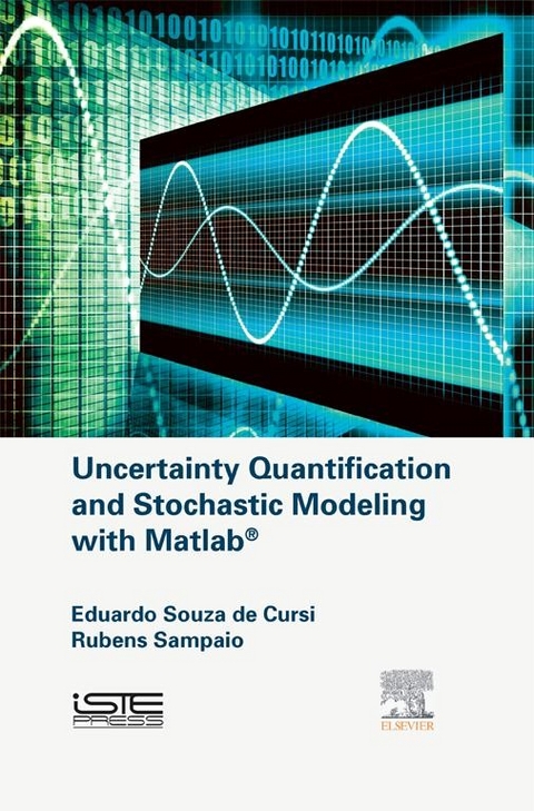
Eduardo Souza De Cursi is Professor at the National Institute for Applied Sciences in Rouen, France, where he is also Dean of International Affairs and Director of the Laboratory for the Optimization and Reliability in Structural Mechanics.
Uncertainty Quantification (UQ) is a relatively new research area which describes the methods and approaches used to supply quantitative descriptions of the effects of uncertainty, variability and errors in simulation problems and models. It is rapidly becoming a field of increasing importance, with many real-world applications within statistics, mathematics, probability and engineering, but also within the natural sciences. Literature on the topic has up until now been largely based on polynomial chaos, which raises difficulties when considering different types of approximation and does not lead to a unified presentation of the methods. Moreover, this description does not consider either deterministic problems or infinite dimensional ones. This book gives a unified, practical and comprehensive presentation of the main techniques used for the characterization of the effect of uncertainty on numerical models and on their exploitation in numerical problems. In particular, applications to linear and nonlinear systems of equations, differential equations, optimization and reliability are presented. Applications of stochastic methods to deal with deterministic numerical problems are also discussed. Matlab illustrates the implementation of these methods and makes the book suitable as a textbook and for self-study. - Discusses the main ideas of Stochastic Modeling and Uncertainty Quantification using Functional Analysis- Details listings of Matlab programs implementing the main methods which complete the methodological presentation by a practical implementation- Construct your own implementations from provided worked examples
Elements of Probability Theory and Stochastic Processes
Abstract
The element which constitutes the foundation of the construction of stochastic algorithms is the concept of random variable, i.e. a function :Ω→R for which individual values X(ω) (ω ∈ Ω) are not available or simply not interesting and we are looking for global information connected to X. For instance, we may consider Ω as the population of a geographic region (country, town, etc) and numerical quantities connected to each individual ω: age, distance or transportation time from a residence to work, level of studies, revenue in the past year, etc. Each of these characteristics may be considered as deterministic, since being perfectly determined for a given individual ω. But to obtain the global information for all the individuals may become expensive (recall the cost of a census) and errors may occur in the process.
Keywords
Data vector
Gaussian samples
Hilbertian structure
Ito Calculus
Linear correlation and affine approximation
Poisson distribution
Quadratic mean convergence
Random variables
Uniform distribution
Wiener process
The element which constitutes the foundation of the construction of stochastic algorithms is the concept of random variable, i.e. a function :Ω→R for which individual values X(ω) (ω ∈ Ω) are not available or simply not interesting and we are looking for global information connected to X.
For instance, we may consider Ω as the population of a geographic region (country, town, etc) and numerical quantities connected to each individual ω: age, distance or transportation time from a residence to work, level of studies, revenue in the past year, etc. Each of these characteristics may be considered as deterministic, since being perfectly determined for a given individual ω. But to obtain the global information for all the individuals may become expensive (recall the cost of a census) and errors may occur in the process. In addition, maybe we are not interested in a particular individual, but only in groups of individuals or in global quantities such as “how many individuals are more than 60 years old?”, “what is the fraction of individuals needing more than one hour of transportation time?”, “how many individuals have finished university”, “how many families have an income lower than …?”. In this case, we may look to the quantities under consideration as random variables.
These examples show that random variables may be obtained by considering numerical characteristics of finite populations. This kind of variable is introduced in section 1.2, and gives a comprehensive introduction to random variables and illustrates their practical use, namely for the numerical calculation of statistics. In the general situation, random variables may be defined on general abstract sets Ω by using the notions of measure and probability (see section 1.7).
1.1 Notation
Let us denote by the set of the natural numbers, and by * the set of the strictly positive real numbers. denotes the set of the real numbers (−∞, +∞) and the notation e refers to the extended real numbers: ⋃{−∞,+∞}. a,b)={x∈R:a<x<b} denotes an open interval of real numbers.
For ∈N*, k={x=(x1,…,xk):xn∈R,1≤n≤k} is the set of the k-tuples formed by real numbers. Analogous notation is used for ek. We denote by |•|p the standard p-norm of k. The standard scalar product of two elements x and y of k is:
x,y)k=∑i=1kxiyi.
When the context is clear enough in order to avoid any confusion, the scalar product on k is simply denote by a point:
.y=(x,y)k.
We will use analogous notation for matrices: A = (Aij)1≤i≤m, 1≤j≤n denotes an m × n-matrix formed by real numbers. The set formed by all the m × n-matrices formed by real numbers is denoted by (m, n). Usually, the elements of k may be seen either as elements of (k, 1) (column vectors) or elements of (1, k) (row vectors). In this text, we consider the elements of k as column vectors, i.e. elements of (k, 1). This allow us to write the product of an m × k matrix A ∈ (m, k) and an element of k, considered as an element of ∈Rk≡M(k,1):
=Ax∈M(m,1)≡Rm.
As usual, we have y = (y1,…, ym), with
i=∑j=1kAijxj.
Sometimes, in order to simplify the expressions, we use the convention on the implicit sum on repeated indexes (called Einstein’s convention) by simply writing yi = Aijxj in this case.
1.2 Numerical characteristics of finite populations
Counts or surveys of the numerical characteristics of finite populations are often generated by censuses, generally made at regular time intervals. For instance, the number of inhabitants, the family income, the type of the house or employment, the school or professional level of the members of the family are some examples of characteristics that are periodically verified.
From the mathematical standpoint, a numerical characteristic X defined on a finite population Ω is a numerical function :Ω→R. As previously observed, an important feature in censuses is that, usually, we are not interested in the particular value X(ω) of the numerical characteristic for a particular individual ω ∈ Ω, but in global quantities connected to X, i.e. in the global behavior of X on the population Ω: what the fraction is of the population having an inferior or superior age to given bounds, what part of the population has revenues inferior or superior to given bounds, etc. Thus, a frequent framework is the following:
1) Ω = {ω1,…, ωN} is a finite population, non-empty set (N ≥ 1)
2) :Ω→R is a numerical characteristic defined on Ω, having as an image a set of k distinct values: X(Ω) = {X1,…, Xk}, Xi ≠ Xj for i ≠ j. Since these values are distinct, they may be arranged in a strictly crescent order: if necessary, we may assume that Xi < Xj for i < j without loss of generality.
3) The inverse image of the value Xi ∈ X(Ω) is the subpopulation Hi = X−1({Xi}) = {ω ∈ Ω : X(ω) = Xi}. The number of elements of Hi is # (Hi) = ni and the relative frequency or probability of Xi is P(X = Xi) = pi = ni/N.
4) Let ⊂R: we define P(A) = nA/N, where nA = # (X−1(A)) is the number of elements of A.
We have:
i=1kpi=1and∑i=1kni=N.
In addition, since the number of elements of Hi ⊂ Ω does not exceed the number of elements N of the global population Ω, we have ni ≤ N. Thus, 0 ≤ pi ≤ 1.
Definition 1.1
mean on a finite population
The mean, or expectation, of X is:
(X)=1N∑n=1NX(ωn).
■
Proposition 1.1
The mean is a linear operation (i.e. E(•) is linear): let :Ω→R and...
| Erscheint lt. Verlag | 9.4.2015 |
|---|---|
| Sprache | englisch |
| Themenwelt | Mathematik / Informatik ► Mathematik ► Algebra |
| Mathematik / Informatik ► Mathematik ► Angewandte Mathematik | |
| Technik ► Maschinenbau | |
| ISBN-10 | 0-08-100471-0 / 0081004710 |
| ISBN-13 | 978-0-08-100471-5 / 9780081004715 |
| Informationen gemäß Produktsicherheitsverordnung (GPSR) | |
| Haben Sie eine Frage zum Produkt? |
Größe: 10,6 MB
Kopierschutz: Adobe-DRM
Adobe-DRM ist ein Kopierschutz, der das eBook vor Mißbrauch schützen soll. Dabei wird das eBook bereits beim Download auf Ihre persönliche Adobe-ID autorisiert. Lesen können Sie das eBook dann nur auf den Geräten, welche ebenfalls auf Ihre Adobe-ID registriert sind.
Details zum Adobe-DRM
Dateiformat: PDF (Portable Document Format)
Mit einem festen Seitenlayout eignet sich die PDF besonders für Fachbücher mit Spalten, Tabellen und Abbildungen. Eine PDF kann auf fast allen Geräten angezeigt werden, ist aber für kleine Displays (Smartphone, eReader) nur eingeschränkt geeignet.
Systemvoraussetzungen:
PC/Mac: Mit einem PC oder Mac können Sie dieses eBook lesen. Sie benötigen eine
eReader: Dieses eBook kann mit (fast) allen eBook-Readern gelesen werden. Mit dem amazon-Kindle ist es aber nicht kompatibel.
Smartphone/Tablet: Egal ob Apple oder Android, dieses eBook können Sie lesen. Sie benötigen eine
Geräteliste und zusätzliche Hinweise
Zusätzliches Feature: Online Lesen
Dieses eBook können Sie zusätzlich zum Download auch online im Webbrowser lesen.
Buying eBooks from abroad
For tax law reasons we can sell eBooks just within Germany and Switzerland. Regrettably we cannot fulfill eBook-orders from other countries.
Größe: 8,1 MB
Kopierschutz: Adobe-DRM
Adobe-DRM ist ein Kopierschutz, der das eBook vor Mißbrauch schützen soll. Dabei wird das eBook bereits beim Download auf Ihre persönliche Adobe-ID autorisiert. Lesen können Sie das eBook dann nur auf den Geräten, welche ebenfalls auf Ihre Adobe-ID registriert sind.
Details zum Adobe-DRM
Dateiformat: EPUB (Electronic Publication)
EPUB ist ein offener Standard für eBooks und eignet sich besonders zur Darstellung von Belletristik und Sachbüchern. Der Fließtext wird dynamisch an die Display- und Schriftgröße angepasst. Auch für mobile Lesegeräte ist EPUB daher gut geeignet.
Systemvoraussetzungen:
PC/Mac: Mit einem PC oder Mac können Sie dieses eBook lesen. Sie benötigen eine
eReader: Dieses eBook kann mit (fast) allen eBook-Readern gelesen werden. Mit dem amazon-Kindle ist es aber nicht kompatibel.
Smartphone/Tablet: Egal ob Apple oder Android, dieses eBook können Sie lesen. Sie benötigen eine
Geräteliste und zusätzliche Hinweise
Zusätzliches Feature: Online Lesen
Dieses eBook können Sie zusätzlich zum Download auch online im Webbrowser lesen.
Buying eBooks from abroad
For tax law reasons we can sell eBooks just within Germany and Switzerland. Regrettably we cannot fulfill eBook-orders from other countries.
aus dem Bereich


