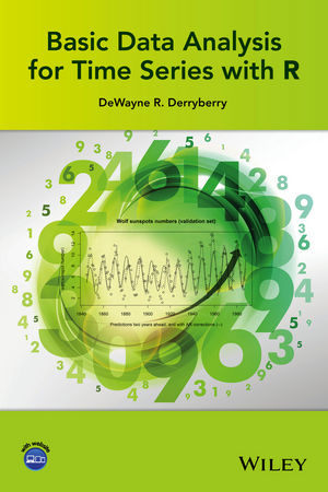
Basic Data Analysis for Time Series with R
John Wiley & Sons Inc (Verlag)
978-1-118-42254-0 (ISBN)
Written at a readily accessible level, Basic Data Analysis for Time Series with R emphasizes the mathematical importance of collaborative analysis of data used to collect increments of time or space. Balancing a theoretical and practical approach to analyzing data within the context of serial correlation, the book presents a coherent and systematic regression-based approach to model selection. The book illustrates these principles of model selection and model building through the use of information criteria, cross validation, hypothesis tests, and confidence intervals.
Focusing on frequency- and time-domain and trigonometric regression as the primary themes, the book also includes modern topical coverage on Fourier series and Akaike's Information Criterion (AIC). In addition, Basic Data Analysis for Time Series with R also features:
Real-world examples to provide readers with practical hands-on experience
Multiple R software subroutines employed with graphical displays
Numerous exercise sets intended to support readers understanding of the core concepts
Specific chapters devoted to the analysis of the Wolf sunspot number data and the Vostok ice core data sets
DeWayne R. Derryberry, PhD, is Associate Professor in the Department of Mathematics and Statistics at Idaho State University. Dr. Derryberry has published more than a dozen journal articles and his research interests include meta-analysis, discriminant analysis with messy data, time series analysis of the relationship between several cancers, and geographically-weighted regression.
PREFACE xv
ACKNOWLEDGMENTS xvii
PART I BASIC CORRELATION STRUCTURES
1 RBasics 3
1.1 Getting Started, 3
1.2 Special R Conventions, 5
1.3 Common Structures, 5
1.4 Common Functions, 6
1.5 Time Series Functions, 6
1.6 Importing Data, 7
Exercises, 7
2 Review of Regression and More About R 8
2.1 Goals of this Chapter, 8
2.2 The Simple(ST) Regression Model, 8
2.2.1 Ordinary Least Squares, 8
2.2.2 Properties of OLS Estimates, 9
2.2.3 Matrix Representation of the Problem, 9
2.3 Simulating the Data from a Model and Estimating the Model Parameters in R, 9
2.3.1 Simulating Data, 9
2.3.2 Estimating the Model Parameters in R, 9
2.4 Basic Inference for the Model, 12
2.5 Residuals Analysis—What Can Go Wrong…, 13
2.6 Matrix Manipulation in R, 15
2.6.1 Introduction, 15
2.6.2 OLS the Hard Way, 15
2.6.3 Some Other Matrix Commands, 16
Exercises, 16
3 The Modeling Approach Taken in this Book and Some Examples of Typical Serially Correlated Data 18
3.1 Signal and Noise, 18
3.2 Time Series Data, 19
3.3 Simple Regression in the Framework, 20
3.4 Real Data and Simulated Data, 20
3.5 The Diversity of Time Series Data, 21
3.6 Getting Data Into R, 24
3.6.1 Overview, 24
3.6.2 The Diskette and the scan() and ts() Functions—New York City Temperatures, 25
3.6.3 The Diskette and the read.table() Function—The Semmelweis Data, 25
3.6.4 Cut and Paste Data to a Text Editor, 26
Exercises, 26
4 Some Comments on Assumptions 28
4.1 Introduction, 28
4.2 The Normality Assumption, 29
4.2.1 Right Skew, 30
4.2.2 Left Skew, 30
4.2.3 Heavy Tails, 30
4.3 Equal Variance, 31
4.3.1 Two-Sample t-Test, 31
4.3.2 Regression, 31
4.4 Independence, 31
4.5 Power of Logarithmic Transformations Illustrated, 32
4.6 Summary, 34
Exercises, 34
5 The Autocorrelation Function And AR(1), AR(2) Models 35
5.1 Standard Models—What are the Alternatives to White Noise?, 35
5.2 Autocovariance and Autocorrelation, 36
5.2.1 Stationarity, 36
5.2.2 A Note About Conditions, 36
5.2.3 Properties of Autocovariance, 36
5.2.4 White Noise, 37
5.2.5 Estimation of the Autocovariance and Autocorrelation, 37
5.3 The acf() Function in R, 37
5.3.1 Background, 37
5.3.2 The Basic Code for Estimating the Autocovariance, 38
5.4 The First Alternative to White Noise: Autoregressive Errors—AR(1), AR(2), 40
5.4.1 Definition of the AR(1) and AR(2) Models, 40
5.4.2 Some Preliminary Facts, 40
5.4.3 The AR(1) Model Autocorrelation and Autocovariance, 41
5.4.4 Using Correlation and Scatterplots to Illustrate the AR(1) Model, 41
5.4.5 The AR(2) Model Autocorrelation and Autocovariance, 41
5.4.6 Simulating Data for AR(m) Models, 42
5.4.7 Examples of Stable and Unstable AR(1) Models, 44
5.4.8 Examples of Stable and Unstable AR(2) Models, 46
Exercises, 49
6 The Moving Average Models MA(1) And MA(2) 51
6.1 The Moving Average Model, 51
6.2 The Autocorrelation for MA(1) Models, 51
6.3 A Duality Between MA(l) And AR(m) Models, 52
6.4 The Autocorrelation for MA(2) Models, 52
6.5 Simulated Examples of the MA(1) Model, 52
6.6 Simulated Examples of the MA(2) Model, 54
6.7 AR(m) and MA(l) model acf() Plots, 54
Exercises, 57
PART II ANALYSIS OF PERIODIC DATA AND MODEL SELECTION
7 Review of Transcendental Functions and Complex Numbers 61
7.1 Background, 61
7.2 Complex Arithmetic, 62
7.2.1 The Number i, 62
7.2.2 Complex Conjugates, 62
7.2.3 The Magnitude of a Complex Number, 62
7.3 Some Important Series, 63
7.3.1 The Geometric and Some Transcendental Series, 63
7.3.2 A Rationale for Euler’s Formula, 63
7.4 Useful Facts About Periodic Transcendental Functions, 64
Exercises, 64
8 The Power Spectrum and the Periodogram 65
8.1 Introduction, 65
8.2 A Definition and a Simplified Form for p(f ), 66
8.3 Inverting p(f ) to Recover the Ck Values, 66
8.4 The Power Spectrum for Some Familiar Models, 68
8.4.1 White Noise, 68
8.4.2 The Spectrum for AR(1) Models, 68
8.4.3 The Spectrum for AR(2) Models, 70
8.5 The Periodogram, a Closer Look, 72
8.5.1 Why is the Periodogram Useful?, 72
8.5.2 Some Na¨ýve Code for a Periodogram, 72
8.5.3 An Example—The Sunspot Data, 74
8.6 The Function spec.pgram() in R, 75
Exercises, 77
9 Smoothers, The Bias-Variance Tradeoff, and the Smoothed Periodogram 79
9.1 Why is Smoothing Required?, 79
9.2 Smoothing, Bias, and Variance, 79
9.3 Smoothers Used in R, 80
9.3.1 The R Function lowess(), 81
9.3.2 The R Function smooth.spline(), 82
9.3.3 Kernel Smoothers in spec.pgram(), 83
9.4 Smoothing the Periodogram for a Series With a Known and Unknown Period, 85
9.4.1 Period Known, 85
9.4.2 Period Unknown, 86
9.5 Summary, 87
Exercises, 87
10 A Regression Model for Periodic Data 89
10.1 The Model, 89
10.2 An Example: The NYC Temperature Data, 91
10.2.1 Fitting a Periodic Function, 91
10.2.2 An Outlier, 92
10.2.3 Refitting the Model with the Outlier Corrected, 92
10.3 Complications 1: CO2 Data, 93
10.4 Complications 2: Sunspot Numbers, 94
10.5 Complications 3: Accidental Deaths, 96
10.6 Summary, 96
Exercises, 96
11 Model Selection and Cross-Validation 98
11.1 Background, 98
11.2 Hypothesis Tests in Simple Regression, 99
11.3 A More General Setting for Likelihood Ratio Tests, 101
11.4 A Subtlety Different Situation, 104
11.5 Information Criteria, 106
11.6 Cross-validation (Data Splitting): NYC Temperatures, 108
11.6.1 Explained Variation, R2, 108
11.6.2 Data Splitting, 108
11.6.3 Leave-One-Out Cross-Validation, 110
11.6.4 AIC as Leave-One-Out Cross-Validation, 112
11.7 Summary, 112
Exercises, 113
12 Fitting Fourier series 115
12.1 Introduction: More Complex Periodic Models, 115
12.2 More Complex Periodic Behavior: Accidental Deaths, 116
12.2.1 Fourier Series Structure, 116
12.2.2 R Code for Fitting Large Fourier Series, 116
12.2.3 Model Selection with AIC, 117
12.2.4 Model Selection with Likelihood Ratio Tests, 118
12.2.5 Data Splitting, 119
12.2.6 Accidental Deaths—Some Comment on Periodic Data, 120
12.3 The Boise River Flow data, 121
12.3.1 The Data, 121
12.3.2 Model Selection with AIC, 122
12.3.3 Data Splitting, 123
12.3.4 The Residuals, 123
12.4 Where Do We Go from Here?, 124
Exercises, 124
13 Adjusting for AR(1) Correlation in Complex Models 125
13.1 Introduction, 125
13.2 The Two-Sample t-Test—UNCUT and Patch-Cut Forest, 125
13.2.1 The Sleuth Data and the Question of Interest, 125
13.2.2 A Simple Adjustment for t-Tests When the Residuals Are AR(1), 128
13.2.3 A Simulation Example, 129
13.2.4 Analysis of the Sleuth Data, 131
13.3 The Second Sleuth Case—Global Warming, A Simple Regression, 132
13.3.1 The Data and the Question, 132
13.3.2 Filtering to Produce (Quasi-)Independent Observations, 133
13.3.3 Simulated Example—Regression, 134
13.3.4 Analysis of the Regression Case, 135
13.3.5 The Filtering Approach for the Logging Case, 136
13.3.6 A Few Comments on Filtering, 137
13.4 The Semmelweis Intervention, 138
13.4.1 The Data, 138
13.4.2 Why Serial Correlation?, 139
13.4.3 How This Data Differs from the Patch/Uncut Case, 139
13.4.4 Filtered Analysis, 140
13.4.5 Transformations and Inference, 142
13.5 The NYC Temperatures (Adjusted), 142
13.5.1 The Data and Prediction Intervals, 142
13.5.2 The AR(1) Prediction Model, 144
13.5.3 A Simulation to Evaluate These Formulas, 144
13.5.4 Application to NYC Data, 146
13.6 The Boise River Flow Data: Model Selection With Filtering, 147
13.6.1 The Revised Model Selection Problem, 147
13.6.2 Comments on R2 and R2 pred, 147
13.6.3 Model Selection After Filtering with a Matrix, 148
13.7 Implications of AR(1) Adjustments and the “Skip” Method, 151
13.7.1 Adjustments for AR(1) Autocorrelation, 151
13.7.2 Impact of Serial Correlation on p-Values, 152
13.7.3 The “skip” Method, 152
13.8 Summary, 152
Exercises, 153
PART III COMPLEX TEMPORAL STRUCTURES
14 The Backshift Operator, the Impulse Response Function, and General ARMA Models 159
14.1 The General ARMA Model, 159
14.1.1 The Mathematical Formulation, 159
14.1.2 The arima.sim() Function in R Revisited, 159
14.1.3 Examples of ARMA(m,l) Models, 160
14.2 The Backshift (Shift, Lag) Operator, 161
14.2.1 Definition of B, 161
14.2.2 The Stationary Conditions for a General AR(m) Model, 161
14.2.3 ARMA(m,l) Models and the Backshift Operator, 162
14.2.4 More Examples of ARMA(m,l) Models, 162
14.3 The Impulse Response Operator—Intuition, 164
14.4 Impulse Response Operator, g(B)—Computation, 165
14.4.1 Definition of g(B), 165
14.4.2 Computing the Coefficients, gj., 165
14.4.3 Plotting an Impulse Response Function, 166
14.5 Interpretation and Utility of the Impulse Response Function, 167
Exercises, 167
15 The Yule–Walker Equations and the Partial Autocorrelation Function 169
15.1 Background, 169
15.2 Autocovariance of an ARMA(m,l) Model, 169
15.2.1 A Preliminary Result, 169
15.2.2 The Autocovariance Function for ARMA(m,l) Models, 170
15.3 AR(m) and the Yule–Walker Equations, 170
15.3.1 The Equations, 170
15.3.2 The R Function ar.yw() with an AR(3) Example, 171
15.3.3 Information Criteria-Based Model Selection Using ar.yw(), 173
15.4 The Partial Autocorrelation Plot, 174
15.4.1 A Sequence of Hypothesis Tests, 174
15.4.2 The pacf() Function—Hypothesis Tests Presented in a Plot, 174
15.5 The Spectrum For Arma Processes, 175
15.6 Summary, 177
Exercises, 178
16 Modeling Philosophy and Complete Examples 180
16.1 Modeling Overview, 180
16.1.1 The Algorithm, 180
16.1.2 The Underlying Assumption, 180
16.1.3 An Example Using an AR(m) Filter to Model MA(3), 181
16.1.4 Generalizing the “Skip” Method, 184
16.2 A Complex Periodic Model—Monthly River Flows, Furnas 1931–1978, 185
16.2.1 The Data, 185
16.2.2 A Saturated Model, 186
16.2.3 Building an AR(m) Filtering Matrix, 187
16.2.4 Model Selection, 189
16.2.5 Predictions and Prediction Intervals for an AR(3) Model, 190
16.2.6 Data Splitting, 191
16.2.7 Model Selection Based on a Validation Set, 192
16.3 A Modeling Example—Trend and Periodicity: CO2 Levels at Mauna Lau, 193
16.3.1 The Saturated Model and Filter, 193
16.3.2 Model Selection, 194
16.3.3 How Well Does the Model Fit the Data?, 197
16.4 Modeling Periodicity with a Possible Intervention—Two Examples, 198
16.4.1 The General Structure, 198
16.4.2 Directory Assistance, 199
16.4.3 Ozone Levels in Los Angeles, 202
16.5 Periodic Models: Monthly, Weekly, and Daily Averages, 205
16.6 Summary, 207
Exercises, 207
PART IV SOME DETAILED AND COMPLETE EXAMPLES
17 Wolf’s Sunspot Number Data 213
17.1 Background, 213
17.2 Unknown Period ⇒ Nonlinear Model, 214
17.3 The Function nls() in R, 214
17.4 Determining the Period, 216
17.5 Instability in the Mean, Amplitude, and Period, 217
17.6 Data Splitting for Prediction, 220
17.6.1 The Approach, 220
17.6.2 Step 1—Fitting One Step Ahead, 222
17.6.3 The AR Correction, 222
17.6.4 Putting it All Together, 223
17.6.5 Model Selection, 223
17.6.6 Predictions Two Steps Ahead, 224
17.7 Summary, 226
Exercises, 226
18 An Analysis of Some Prostate and Breast Cancer Data 228
18.1 Background, 228
18.2 The First Data Set, 229
18.3 The Second Data Set, 232
18.3.1 Background and Questions, 232
18.3.2 Outline of the Statistical Analysis, 233
18.3.3 Looking at the Data, 233
18.3.4 Examining the Residuals for AR(m) Structure, 235
18.3.5 Regression Analysis with Filtered Data, 238
Exercises, 243
19 Christopher Tennant/Ben Crosby Watershed Data 245
19.1 Background and Question, 245
19.2 Looking at the Data and Fitting Fourier Series, 246
19.2.1 The Structure of the Data, 246
19.2.2 Fourier Series Fits to the Data, 246
19.2.3 Connecting Patterns in Data to Physical Processes, 246
19.3 Averaging Data, 248
19.4 Results, 250
Exercises, 250
20 Vostok Ice Core Data 251
20.1 Source of the Data, 251
20.2 Background, 252
20.3 Alignment, 253
20.3.1 Need for Alignment, and Possible Issues Resulting from Alignment, 253
20.3.2 Is the Pattern in the Temperature Data Maintained?, 254
20.3.3 Are the Dates Closely Matched?, 254
20.3.4 Are the Times Equally Spaced?, 255
20.4 A Na¨ýve Analysis, 256
20.4.1 A Saturated Model, 256
20.4.2 Model Selection, 258
20.4.3 The Association Between CO2 and Temperature Change, 258
20.5 A Related Simulation, 259
20.5.1 The Model and the Question of Interest, 259
20.5.2 Simulation Code in R, 260
20.5.3 A Model Using all of the Simulated Data, 261
20.5.4 A Model Using a Sample of 283 from the Simulated Data, 262
20.6 An AR(1) Model for Irregular Spacing, 265
20.6.1 Motivation, 265
20.6.2 Method, 266
20.6.3 Results, 266
20.6.4 Sensitivity Analysis, 267
20.6.5 A Final Analysis, Well Not Quite, 268
20.7 Summary, 269
Exercises, 270
Appendix A Using Datamarket 273
A.1 Overview, 273
A.2 Loading a Time Series in Datamarket, 277
A.3 Respecting Datamarket Licensing Agreements, 280
Appendix B AIC is PRESS! 281
B.1 Introduction, 281
B.2 PRESS, 281
B.3 Connection to Akaike’s Result, 282
B.4 Normalization and R2, 282
B.5 An example, 283
B.6 Conclusion and Further Comments, 283
Appendix C A 15-Minute Tutorial on Nonlinear Optimization 284
C.1 Introduction, 284
C.2 Newton’s Method for One-Dimensional Nonlinear Optimization, 284
C.3 A Sequence of Directions, Step Sizes, and a Stopping Rule, 285
C.4 What Could Go Wrong?, 285
C.5 Generalizing the Optimization Problem, 286
C.6 What Could Go Wrong—Revisited, 286
C.7 What Can be Done?, 287
REFERENCES 291
INDEX 293
| Verlagsort | New York |
|---|---|
| Sprache | englisch |
| Maße | 160 x 244 mm |
| Gewicht | 649 g |
| Themenwelt | Mathematik / Informatik ► Mathematik ► Computerprogramme / Computeralgebra |
| Mathematik / Informatik ► Mathematik ► Wahrscheinlichkeit / Kombinatorik | |
| ISBN-10 | 1-118-42254-6 / 1118422546 |
| ISBN-13 | 978-1-118-42254-0 / 9781118422540 |
| Zustand | Neuware |
| Informationen gemäß Produktsicherheitsverordnung (GPSR) | |
| Haben Sie eine Frage zum Produkt? |
aus dem Bereich


