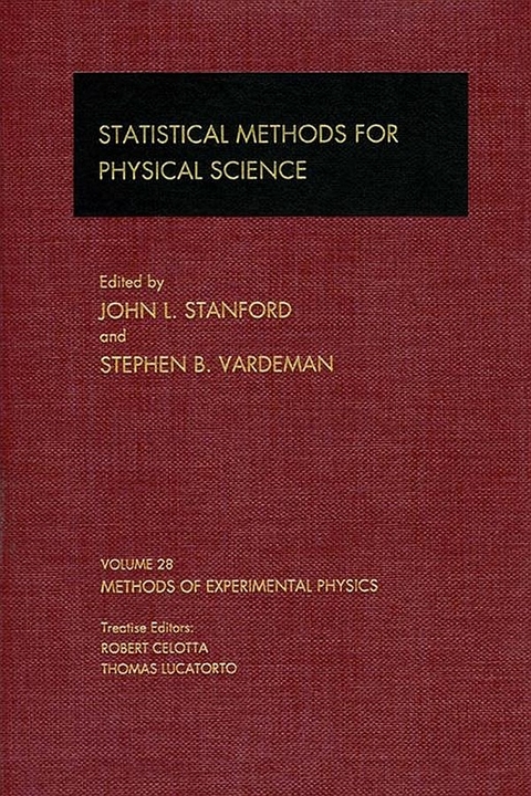
Statistical Methods for Physical Science (eBook)
542 Seiten
Elsevier Science (Verlag)
978-0-08-086016-9 (ISBN)
Key Features
* Examines basic probability, including coverage of standard distributions, time series models, and Monte Carlo methods
* Describes statistical methods, including basic inference, goodness of fit, maximum likelihood, and least squares
* Addresses time series analysis, including filtering and spectral analysis
* Includes simulations of physical experiments
* Features applications of statistics to atmospheric physics and radio astronomy
* Covers the increasingly important area of modern statistical computing
This volume of Methods of Experimental Physics provides an extensive introduction to probability and statistics in many areas of the physical sciences, with an emphasis on the emerging area of spatial statistics. The scope of topics covered is wide-ranging-the text discusses a variety of the most commonly used classical methods and addresses newer methods that are applicable or potentially important. The chapter authors motivate readers with their insightful discussions. - Examines basic probability, including coverage of standard distributions, time series models, and Monte Carlo methods- Describes statistical methods, including basic inference, goodness of fit, maximum likelihood, and least squares- Addresses time series analysis, including filtering and spectral analysis- Includes simulations of physical experiments- Features applications of statistics to atmospheric physics and radio astronomy- Covers the increasingly important area of modern statistical computing
Front Cover 1
Statistical Methods for Physical Science 4
Copyright Page 5
Contents 6
Contributors 14
Preface 16
Chapter 1. Introduction to Probability Modeling 22
1.1. Probability in Experimental Physics 22
1.2. Defining Probability 25
1.3. Elements of Probability Theory 29
1.4. Modeling Measurement 48
References 55
Chapter 2. Common Univariate Distributions 56
2.1. Introduction 56
2.2. Discrete Probability Mass Functions 56
2.3. Continuous Probability Distributions 67
References 82
Chapter 3. Random Process Models 84
3.1. Introduction 84
3.2. Probability Models for Time Series 85
3.3. Spectral Properties of Random Processes 99
3.4. Point Process Models 104
3.5. Further Reading 112
References 112
Chapter 4. Models for Spatial Processes 114
4.1. Introduction 114
4.2. Geostatistical Models 116
4.3. Lattice Models 124
4.4. Spatial Point Processes 133
4.5. Some Final Remarks 143
References 144
Chapter 5. Monte Carlo Methods 146
5.1. Introduction 146
5.2. Continuous Distributions 150
5.3. Discrete Distributions 155
5.4. Multivariate Distributions 157
5.5. Monte Carlo Integration 161
5.6. Time Series 163
5.7. Spatial Processes 167
5.8. Markov Random Fields 171
5.9. Point Processes 173
5.10. Further Reading 174
References 174
Chapter 6. Basic Statistical Inference 176
6.1. Introduction 176
6.2. Point Estimation 181
6.3. Interval Estimation 186
6.4. Statistical Tests 200
6.5. Beyond Basic Statistical Inference 204
References 206
Chapter 7. Methods for Assessing Distributional Assumptions in One- and Two-Sample Problems 208
7.1. Introduction 208
7.2. Chi-Squared Tests 209
7.3. Quantile–Quantile (Q-Q) Plots 213
7.4. Formal Test Procedures 222
7.5. Extensions to Censored Data 225
7.6. Two-Sample Comparisons 228
References 230
Chapter 8. Maximum Likelihood Methods for Fitting Parametric Statistical Models 232
8.1. Introduction 232
8.2. Data from Continuous Models 235
8.3. General Method and Application to the Exponential Distribution (a One-Parameter Model) 242
8.4. Fitting the Weibull with Left-Censored Observations (a Two- Parameter Model) 251
8.5. Fitting the Limited Failure Population Model (a Three Parameter Model) 256
8.6. Some Other Applications 260
8.7. Other Topics and Sources of Additional Information 261
References 264
Chapter 9: Least Squares 266
9.1. Statistical Modeling 266
9.2. The Error Process Viewed Statistically 273
9.3. Least Squares Fitting 275
9.4. Statistical Properties of Least Squares Estimates 277
9.5. Statistical Inference 282
9.6. Diagnostics 287
9.7. Errors in the Regressors 298
References 301
Chapter 10. Filtering and Data Preprocessing for Time Series Analysis 304
10.1. Filtering Time Series 304
10.2. Data Preprocessing for Spectral Analysis 318
10.3. Imperfectly Sampled Time Series 326
References 331
Chapter 11. Spectral Analysis of Univariate and Bivariate Time Series 334
11.1. Introduction 334
11.2. Univariate Time Series 337
11.3. Bivariate Time Series 361
References 368
Chapter 12. Weak Periodic Signals in Point Process Data 370
12.1. Introduction 370
12.2. White Noise and Light Curves 372
12.3. Tests for Uniformity of Phase 373
12.4. dc Excess vs. Periodic Strength 382
12.5. Frequency Searches 385
12.6. Multiple Data Sets 388
References 393
Chapter 13. Statistical Analysis of Spatial Data 396
13.1. Introduction 396
13.2. Sulfate Deposition Data 397
13.3. The Geostatistical Model 399
13.4. Estimation of First-Order Structure 402
13.5. Estimation of Second-Order Structure 409
13.6. Spatial Prediction (Kriging) 417
13.7. Extensions and Related Issues 419
References 421
Chapter 14. Bayesian Methods 424
14.1. Bayesian Statistical Inference 424
14.2. The Prior Distribution 428
14.3. Bayesian Estimation 434
14.4. Examples 435
14.5. The Gibbs Sampler 448
References 451
Chapter 15. Simulation of Physical Systems 454
15.1. Introduction 454
15.2. Basic Techniques in Simulation 457
15.3. Finding Nonalgebraic Solutions 461
15.4. Simulation of Experiments 465
15.5. Validity Testing and Analysis 471
15.6. Improbable Events and Small Effects 474
15.7. Simulations within Simulations 475
References 476
Chapter 16. Field (Map) Statistics 478
16.1. Introduction 478
16.2. Field Statistic Assessment by Monte Carlo Simulation 483
16.3. Example One: Atmospheric Temperature Fields 487
16.4. Example Two: Global Ozone Data Fields 492
16.5. Example Three: Cross Correlation between Ozone and Solar Flux Time Series 496
16.6. Higher Dimensions 499
16.7. Summary 499
References 499
Chapter 17. Modern Statistical Computing and Graphics 502
17.1. Introduction 502
17.2. Statistical Computing Environments 503
17.3. Computational Methods in Statistics 509
17.4. Computer-Intensive Statistical Methods 512
17.5. Application: Differential Equation Models 522
17.6. Graphical Methods 530
17.7. Conclusion 537
References 538
Tables 542
Index 552
Introduction to Probability Modeling
William R. Leo Astral Geneva, Switzerland
To understand probability, I think you need to be older.
-M. Schöunburg
1.1 Probability in Experimental Science
Historically, the invention of probability theory is generally attributed to Pascal and Femiat, who first developed it to treat a narrow domain of problems connected with games of chance. Progress in the ensuing centuries, however, has widened its applications such that today almost all disciplines, be they the physical sciences, engineering, the social sciences, economics, etc., are touched in some way or another. In physics, for example, probability appears in an extremely fundamental role in quantum theory and in statistical mechanics, where it is used to describe the ultimate behavior of matter. Notwithstanding its importance to modern physical theory, however, probability also plays an almost equally fundamental role on the experimental side—for it can be said that probability is one of the truly basic tools of the experimental sciences, without which many results would not have been possible.
Modem science, of course, is based on active experimentation; that is, observation and measurement. This is the fundamental means by which new knowledge is acquired. But it becomes evident to anyone who has ever performed experiments that all measurements are fraught with uncertainty or “errors,” which limit the conclusions that can be drawn. (The term errors here is the one used most often by scientists to refer to experimental unceilainties, and its meaning should not be confused with that of “making a mistake. ”) The questions that inevitably arise then are these: How is one to handle these uncertainties? Can one still draw any real conclusions from the data? How much confidence can one have in the results? Moreover, given the data, how does one compare them to results from other experiments? Are they different or consistent? Here the problem is not so much the final result itself but the errors incurred. This implies that a common quantitative measure and “language” are necessary to describe the errors. Finally, given that there are errors in all measurements, is it possible to plan and design one’s experiment so that it will give meaningful results? Here again, a quantitative procedure is necessary.
The answer to these questions comes from recognizing that measurement and observational errors are in fact random phenomena and that they can be modelled and interpreted using the theory of probability. The consequence is that “uncertainty,” an intuitive notion, can now be quantified and treated with the mathematical apparatus already developed in probability and in statistics. Ultimately, this allows the confidence one can have in the result, and therefore the meaningfulness of the experiment, to be gauged in a quantitative way. At the same time, the mathematical theory provides a standard framework in which different measurements or observations of the same phenomenon can be compared in a consistent manner.
The notion of probability is familiar to most people, however, the mathematical theory of probability and its application are much less so. Indeed, nowhere in mathematics are more errors (i.e., mistakes!) in reasoning made more often than in probability theory (see, for example, Chapters 1–2 of [1] and Section VI, [2]). Applying probability in a consistent manner requires, in fact, a rather radical change in conceptual thinking.
History gives us some interesting illustrations of this, one of which is the work of Tobias Mayer, who in the mid-18th century successfully treated the problem of the libration of the moon. The term libration refers to slow, oscillatory movements made by the moon’s body such that parts of its face appear and disappear from view. There are, in fact, several movements along different axes that, over an extended period of time, allow about 60% of the moon’s surface to be seen from the earth. The causes of these effects were known at the time of Tobias Mayer, but the problem was to account for these movements either by a mathematical equation or a set of lunar tables. Indeed, a solution was of particular commercial and military value for detailed knowledge of the moon’s different motions could serve as a navigational aide to ships at sea.
Thus, in 1748, Johann Tobias Mayer, an already well-known cartographer and practical astronomer, undertook the study of the libration problem. After making observations of the moon for more than a year, Mayer came up with a method for determining various characteristics of these movements. A critical pm of this solution was to find the relationship between the natural coordinate system of the moon as defined by its axis of rotation and equator and the astronomer’s system defined by the plane of the earth’s orbit about the sun (ecliptic). To do this, Mayer focused his observations on the position of the crater Manilius and derived a relation between the two reference systems involving six parameters, three of which were unknown constants and three of which varied with the moon’s motion, but could be measured. To solve for these unknowns, therefore, Mayer needed only to make three day’s worth of observations. He did better than this, however, and made observations over a period of 27 days.
Keeping in mind that the discovery of the least squares principle (see Chapter 9) was still a half-century off, Mayer was thus faced with the dilemma of having 27 inconsistent equations for his three unknowns; that is, if he attempted to solve for the unknowns by just taking three of the equations, different results would be obtained depending on which three equations he chose. The inconsistencies, of course, were due to the observational errors, an effect well known to the scientists and mathematicians of the time, but for which no one had a solution. It was here that Mayer came up with a remarkable idea. From his own practical experience, Mayer knew intuitively that adding observations made under similar conditions could actually reduce the errors incurred. Using this notion, he divided his equations into three groups of nine similar equations, added the equations in each group and solved for his unknowns. Simple1 as that!
The point, however, is that Mayer essentially thought of his errors as random phenomena, although he had no clear concept of probability, so that adding data could actually lead to a cancellation of the errors and a reduction in the overall uncertainty. This was totally contrary to the view of the times, which focused on the maximum possible error (as opposed to the probable error) that could occur when data were manipulated. From this viewpoint, adding data would only increase the final errors, since it wouldjust cumulate the maximum possible error of each datum. Such a large final error is possible under the probabilistic view but highly improbable.
Interestingly enough history also provides a “control experiment” to prove the point. Only one year prior to Mayer’s work, Leonhard Euler, undoubtedly one of the greatest mathematicians of all time, reported his work on the problem of “inequalities” in the orbits of Jupiter and Samm. These effects were thought to be due to the two planets' mutual attraction, an instance of what today is called the three-body problem. Formulating a mathematical equation for the longitudinal position of Saturn that took into account the attraction of both the sun and Jupiter, Euler sought to provide some test of his calculation by using some actual data (not of his own taking). After making a number of approximations to linearize his formula, he ended up with 75 equations for six unknowns. He thus faced a problem analytically similar to Tobias Mayer’s, although on a somewhat larger scale.
Here, however, Euler failed to make the conceptual jump that Mayer made. Indeed, whereas Mayer made his own measurements and thus had an intuitive feeling for the uncertainties involved, Euler, a pure mathematician dealing with data that he did not take, had no basis for even imagining the random nature of measurement errors. Euler was thus left to grope for a solution that he never found. His theoretical work, was nevertheless a significant contribution to celestial mechanics, and in recognition, he was awarded the 1748 prize offered by the Academy of Sciences in Paris. Further details conceming Tobias Mayer’s and Leonhard Euler’s work may be found in [3].
These historical accounts illustrate the paradigm shift that the application of probability theory required in its early stages, but even today dealing with probability theory still requires a conceptual change that is underestimated by most people. Indeed, to think probabilistically essentially requires giving up certainty in everything that is done, as we will see later on. This is also complicated by a good deal of confusion over the meaning of certain terms—beginning with the expressions probability and probability theory themselves. We will attempt to clarify these points in the next sections.
1.2 Defining Probability
In applying probability theory it is necessary to distinguish between two distinct problems: the modeling of random processes...
| Erscheint lt. Verlag | 13.12.1994 |
|---|---|
| Sprache | englisch |
| Themenwelt | Mathematik / Informatik ► Mathematik ► Statistik |
| Naturwissenschaften ► Chemie | |
| Naturwissenschaften ► Physik / Astronomie ► Thermodynamik | |
| Technik ► Maschinenbau | |
| ISBN-10 | 0-08-086016-8 / 0080860168 |
| ISBN-13 | 978-0-08-086016-9 / 9780080860169 |
| Haben Sie eine Frage zum Produkt? |
Kopierschutz: Adobe-DRM
Adobe-DRM ist ein Kopierschutz, der das eBook vor Mißbrauch schützen soll. Dabei wird das eBook bereits beim Download auf Ihre persönliche Adobe-ID autorisiert. Lesen können Sie das eBook dann nur auf den Geräten, welche ebenfalls auf Ihre Adobe-ID registriert sind.
Details zum Adobe-DRM
Dateiformat: EPUB (Electronic Publication)
EPUB ist ein offener Standard für eBooks und eignet sich besonders zur Darstellung von Belletristik und Sachbüchern. Der Fließtext wird dynamisch an die Display- und Schriftgröße angepasst. Auch für mobile Lesegeräte ist EPUB daher gut geeignet.
Systemvoraussetzungen:
PC/Mac: Mit einem PC oder Mac können Sie dieses eBook lesen. Sie benötigen eine
eReader: Dieses eBook kann mit (fast) allen eBook-Readern gelesen werden. Mit dem amazon-Kindle ist es aber nicht kompatibel.
Smartphone/Tablet: Egal ob Apple oder Android, dieses eBook können Sie lesen. Sie benötigen eine
Geräteliste und zusätzliche Hinweise
Buying eBooks from abroad
For tax law reasons we can sell eBooks just within Germany and Switzerland. Regrettably we cannot fulfill eBook-orders from other countries.
aus dem Bereich


