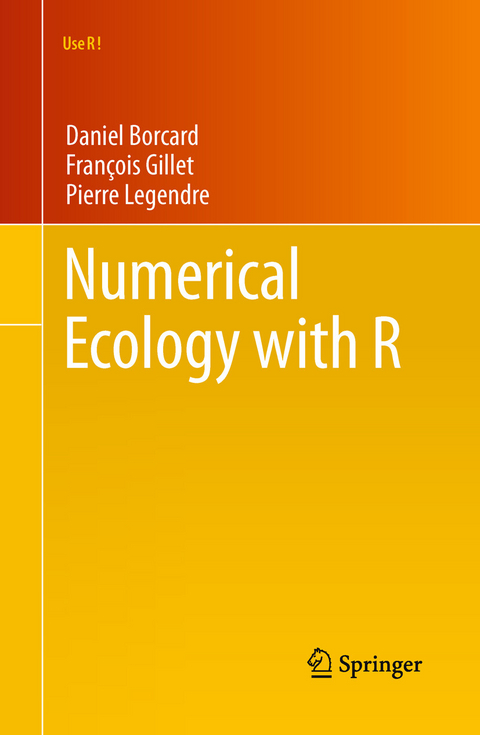
Numerical Ecology with R (eBook)
XII, 306 Seiten
Springer New York (Verlag)
978-1-4419-7976-6 (ISBN)
Numerical Ecology with R provides a long-awaited bridge between a textbook in Numerical Ecology and the implementation of this discipline in the R language. After short theoretical overviews, the authors accompany the users through the exploration of the methods by means of applied and extensively commented examples. Users are invited to use this book as a teaching companion at the computer. The travel starts with exploratory approaches, proceeds with the construction of association matrices, then addresses three families of methods: clustering, unconstrained and canonical ordination, and spatial analysis. All the necessary data files, the scripts used in the chapters, as well as the extra R functions and packages written by the authors, can be downloaded from a web page accessible through the Springer web site(http://adn.biol.umontreal.ca/-numericalecology/numecolR/).
This book is aimed at professional researchers, practitioners, graduate students and teachers in ecology, environmental science and engineering, and in related fields such as oceanography, molecular ecology, agriculture and soil science, who already have a background in general and multivariate statistics and wish to apply this knowledge to their data using the R language, as well as people willing to accompany their disciplinary learning with practical applications. People from other fields (e.g. geology, geography, paleoecology, phylogenetics, anthropology, the social and education sciences, etc.) may also benefit from the materials presented in this book.
The three authors teach numerical ecology, both theoretical and practical, to a wide array of audiences, in regular courses in their Universities and in short courses given around the world. Daniel Borcard is lecturer of Biostatistics and Ecology and researcher in Numerical Ecology at Université de Montréal, Québec, Canada. François Gillet is professor of Community Ecology and Ecological Modelling at Université de Franche-Comté, Besançon, France. Pierre Legendre is professor of Quantitative Biology and Ecology at Université de Montréal, Fellow of the Royal Society of Canada, and ISI Highly Cited Researcher in Ecology/Environment.
The three authors teach numerical ecology, both theoretical and practical, to a wide array of audiences, in regular courses in their Universities and in short courses given around the world. Daniel Borcard is lecturer of Biostatistics and Ecology and researcher in Numerical Ecology at Université de Montréal, Québec, Canada. François Gillet is professor of Community Ecology and Ecological Modelling at Université de Franche-Comté, Besançon, France. Pierre Legendre is professor of Quantitative Biology and Ecology at Université de Montréal, Fellow of the Royal Society of Canada, and ISI Highly Cited Researcher in Ecology/Environment.
Numerical Ecology with R provides a long-awaited bridge between a textbook in Numerical Ecology and the implementation of this discipline in the R language. After short theoretical overviews, the authors accompany the users through the exploration of the methods by means of applied and extensively commented examples. Users are invited to use this book as a teaching companion at the computer. The travel starts with exploratory approaches, proceeds with the construction of association matrices, then addresses three families of methods: clustering, unconstrained and canonical ordination, and spatial analysis. All the necessary data files, the scripts used in the chapters, as well as the extra R functions and packages written by the authors, can be downloaded from a web page accessible through the Springer web site (http://www.bio.umontreal.ca/numecolR/).This book is aimed at professional researchers, practitioners, graduate students and teachers in ecology, environmental science and engineering, and in related fields such as oceanography, molecular ecology, agriculture and soil science, who already have a background in general and multivariate statistics and wish to apply this knowledge to their data using the R language, as well as people willing to accompany their disciplinary learning with practical applications. People from other fields (e.g. geology, geography, paleoecology, phylogenetics, anthropology, the social and education sciences, etc.) may also benefit from the materials presented in this book. The three authors teach numerical ecology, both theoretical and practical, to a wide array of audiences, in regular courses in their Universities and in short courses given around the world. Daniel Borcard is lecturer of Biostatistics and Ecology and researcher in Numerical Ecology at Universite de Montreal, Quebec, Canada. Francois Gillet is professor of Community Ecology and Ecological Modelling at Universite de Franche-Comte, Besancon, France. Pierre Legendre is professor of Quantitative Biology and Ecology at Universite de Montreal, Fellow of the Royal Society of Canada, and ISI Highly Cited Researcher in Ecology/Environment.
The three authors teach numerical ecology, both theoretical and practical, to a wide array of audiences, in regular courses in their Universities and in short courses given around the world. Daniel Borcard is lecturer of Biostatistics and Ecology and researcher in Numerical Ecology at Université de Montréal, Québec, Canada. François Gillet is professor of Community Ecology and Ecological Modelling at Université de Franche-Comté, Besançon, France. Pierre Legendre is professor of Quantitative Biology and Ecology at Université de Montréal, Fellow of the Royal Society of Canada, and ISI Highly Cited Researcher in Ecology/Environment.
Preface 6
Contents 8
Chapter 1: Introduction 14
1.1 Why Numerical Ecology? 14
1.2 Why R? 15
1.3 Readership and Structure of the Book 15
1.4 How to Use This Book 16
1.5 The Data Sets 17
1.5.1 The Doubs Fish Data 17
1.5.2 The Oribatid Mite Data 18
1.6 A Quick Reminder about Help Sources 20
1.7 Now It Is Time 20
Chapter 2: Exploratory Data Analysis 21
2.1 Objectives 21
2.2 Data Exploration 21
2.2.1 Data Extraction 21
2.2.2 Species Data: First Contact 22
2.2.3 Species Data: A Closer Look 24
2.2.4 Species Data Transformation 30
2.2.5 Environmental Data 36
The Code It Yourself corner #1 35
2.3 Conclusion 42
Chapter 3: Association Measures and Matrices 43
3.1 Objectives 43
3.2 The Main Categories of Association Measures (Short Overview) 43
3.2.1 Q Mode and R Mode 44
3.2.2 Symmetrical or Asymmetrical Coefficients in Q Mode: The Double-Zero Problem 44
3.2.3 Association Measures for Qualitative or Quantitative Data 45
3.2.4 To Summarize… 45
3.3 Q Mode: Computing Distance Matrices Among Objects 46
3.3.1 Q Mode: Quantitative Species Data 46
3.3.2 Q Mode: Binary (Presence–Absence) Species Data 48
3.3.3 Q Mode: Quantitative Data (Excluding Species Abundances) 53
3.3.4 Q Mode: Binary Data (Excluding Species Presence–Absence Data) 55
3.3.5 Q Mode: Mixed Types, Including Categorical (Qualitative Multiclass) Variables 56
The Code It Yourself corner #2 52
3.4 R Mode: Computing Dependence Matrices Among Variables 58
3.4.1 R Mode: Species Abundance Data 58
3.4.2 R Mode: Species Presence–Absence Data 59
3.4.3 R Mode: Quantitative and Ordinal Data (Other than Species Abundances) 59
3.4.4 R Mode: Binary Data (Other than Species Abundance Data) 61
3.5 Pre-transformations for Species Data 62
3.6 Conclusion 62
Chapter 4: Cluster Analysis 64
4.1 Objectives 64
4.2 Clustering Overview 64
4.3 Hierarchical Clustering Based on Links 67
4.3.1 Single Linkage Agglomerative Clustering 67
4.3.2 Complete Linkage Agglomerative Clustering 68
4.4 Average Agglomerative Clustering 70
4.5 Ward’s Minimum Variance Clustering 72
4.6 Flexible Clustering 74
4.7 Interpreting and Comparing Hierarchical Clustering Results 74
4.7.1 Introduction 74
4.7.2 Cophenetic Correlation 74
4.7.3 Looking for Interpretable Clusters 76
4.7.3.1 Graph of the Fusion Level Values 77
4.7.3.2 Graphs of Silhouette Widths 80
4.7.3.3 Comparison Between the Distance Matrix and Binary Matrices Representing Partitions 82
4.7.3.4 Silhouette Plot of the Final Partition 84
4.7.3.5 Final Dendrogram with Graphical Options 85
4.7.3.6 Spatial Plot of the Clustering Result 87
4.7.3.7 Heat Map and Ordered Community Table 88
4.8 Non-hierarchical Clustering 90
4.8.1 k-Means Partitioning 91
4.8.2 Partitioning Around Medoids 95
4.9 Comparison with Environmental Data 98
4.9.1 Comparing a Typology with External Data (ANOVA Approach) 99
4.9.2 Comparing Two Typologies (Contingency Table Approach) 102
4.10 Species Assemblages 102
4.10.1 Simple Statistics on Group Contents 102
4.10.2 Kendall’s W Coefficient of Concordance 103
4.10.3 Species Assemblages in Presence–Absence Data 106
4.10.4 IndVal: Species Indicator Values 108
4.11 Multivariate Regression Trees: Constrained Clustering 110
4.11.1 Introduction 110
4.11.2 Computation (Principle) 110
4.11.2.1 Constrained Partitioning of the Data 110
4.11.2.2 Cross-Validation of the Partitions and Pruning of the Tree 111
4.11.2.3 MRT Procedure 112
4.11.3 Application Using Packages mvpart and MVPARTwrap 113
4.11.4 Combining MRT and IndVal 118
4.11.5 MRT as a “Chronological” Clustering Method 119
4.12 A Very Different Approach: Fuzzy Clustering 121
4.12.1 Fuzzy c-Means Clustering Using cluster’s Function fanny() 121
4.13 Conclusion 125
Chapter 5: Unconstrained Ordination 126
5.1 Objectives 126
5.2 Ordination Overview 126
5.2.1 Multidimensional Space 126
5.2.2 Ordination in Reduced Space 127
5.3 Principal Component Analysis 128
5.3.1 Overview 128
5.3.2 PCA on the Environmental Variables of the Doubs Data Set Using rda() 129
5.3.2.1 Preparation of the Data 129
5.3.2.2 PCA on a Correlation Matrix 130
5.3.2.3 Extracting, Interpreting and Plotting Results from a vegan Ordination Output Object 132
Eigenvalues 132
Biplots of Sites and Variables 135
5.3.2.4 Combining Clustering and Ordination Results 138
5.3.3 PCA on Transformed Species Data 139
5.3.4 Domain of Application of PCA 141
5.3.5 PCA Using Function PCA() 142
5.4 Correspondence Analysis 143
5.4.1 Introduction 143
5.4.2 CA Using Function cca() of Package vegan 144
5.4.2.1 Running the Analysis and Drawing the Biplots 144
5.4.2.2 Passive (Post Hoc) Explanation of Axes Using Environmental Variables 147
5.4.2.3 Reordering the Data Table on the Basis of an Ordination Axis 149
5.4.3 CA Using Function CA() 149
5.4.4 Arch Effect and Detrended Correspondence Analysis 150
5.4.5 Multiple Correspondence Analysis 151
5.5 Principal Coordinate Analysis 151
5.5.1 Introduction 151
5.5.2 Application to the Doubs Data Set Using cmdscale and vegan 152
5.5.3 Application to the Doubs Data Set Using pcoa() 154
5.6 Nonmetric Multidimensional Scaling 156
5.6.1 Introduction 156
5.6.2 Application to the Fish Data 157
5.7 Handwritten Ordination Function 160
Chapter 6: Canonical Ordination 163
6.1 Objectives 163
6.2 Canonical Ordination Overview 164
6.3 Redundancy Analysis 164
6.3.1 Introduction 164
6.3.2 RDA of the Doubs River Data 166
6.3.2.1 Preparation of the Data 166
6.3.2.2 RDA Using vegan 167
6.3.2.3 Retrieving, Interpreting and Plotting Results from a vegan RDA Output Object 172
6.3.2.4 Permutation Tests of RDA Results 179
6.3.2.5 Partial RDA 181
6.3.2.6 Forward Selection of Explanatory Variables 185
6.3.2.7 Variation Partitioning 190
6.3.2.8 RDA as a Tool for Multivariate ANOVA 195
6.3.2.9 Distance-Based Redundancy Analysis 198
6.3.2.10 Nonlinear Relationships in RDA 200
6.3.3 A Hand-Written RDA Function 205
6.4 Canonical Correspondence Analysis 208
6.4.1 Introduction 208
6.4.2 CCA of the Doubs Data 209
6.4.2.1 CCA Using vegan 209
6.4.2.2 CCA Triplot 210
6.4.2.3 Permutation Tests in CCA, Forward Selection and Parsimonious CCA 215
6.4.2.4 Three-Dimensional Interactive Plots 216
6.5 Linear Discriminant Analysis 217
6.5.1 Introduction 217
6.5.2 Discriminant Analysis Using lda() 218
6.6 Other Asymmetrical Analyses 220
6.7 Symmetrical Analysis of Two (or More) Data Sets 221
6.8 Canonical Correlation Analysis 221
6.8.1 Introduction 221
6.8.2 Canonical Correlation Analysis using CCorA 222
6.9 Co-inertia Analysis 224
6.9.1 Introduction 224
6.9.2 Co-inertia Analysis Using ade4 225
6.10 Multiple Factor Analysis 228
6.10.1 Introduction 228
6.10.2 Multiple Factor Analysis Using FactoMineR 229
6.11 Conclusion 234
Chapter 7: Spatial Analysis of Ecological Data 236
7.1 Objectives 236
7.2 Spatial Structures and Spatial Analysis: A Short Overview 237
7.2.1 Introduction 237
7.2.2 Induced Spatial Dependence and Spatial Autocorrelation 238
7.2.3 Spatial Scale 239
7.2.4 Spatial Heterogeneity 240
7.2.5 Spatial Correlation or Autocorrelation Functions and Spatial Correlograms 241
7.2.6 Testing for the Presence of Spatial Correlation: Conditions 245
7.2.7 Modelling Spatial Structures 247
7.3 Multivariate Trend-Surface Analysis 247
7.3.1 Introduction 247
7.3.2 Trend-Surface Analysis in Practice 248
7.4 Eigenvector-Based Spatial Variables and Spatial Modelling 252
7.4.1 Introduction 252
7.4.2 Classical Distance-Based MEM, Formerly Called Principal Coordinates of Neighbour Matrices 253
7.4.2.1 Introduction 253
7.4.2.2 PCNM Variables on Regular Sampling Designs 254
7.4.2.3 PCNM Analysis of the Mite Data 257
7.4.2.4 Hassle-Free PCNM Analysis: Function quickPCNM() 266
7.4.2.5 Combining PCNM Analysis and Variation Partitioning 267
7.4.3 MEM in a Wider Context: Weights Other than Geographic Distances 272
7.4.3.1 Introduction 272
7.4.3.2 MEM Analysis of the Mite Data 274
7.4.3.3 Other Types of Connectivity Matrices 281
7.4.3.4 Controlling for Spatial Correlation Using MEM 286
7.4.3.5 MEM on Sampling Designs with Nested Spatial Scales 287
7.4.4 MEM with Positive or Negative Spatial Correlation: Which Ones Should Be Used? 287
7.4.5 Asymmetric Eigenvector Maps: When Directionality Matters 288
7.4.5.1 Introduction 288
7.4.5.2 Principle of the Method 289
7.5 Another Way to Look at Spatial Structures: Multiscale Ordination 294
7.5.1 Principle 294
7.5.2 Application to the Mite Data: Exploratory Approach 295
7.5.3 Application to the Detrended Mite and Environmental Data 298
7.6 Conclusion 301
Bibliographical References 302
Index 310
| Erscheint lt. Verlag | 7.1.2011 |
|---|---|
| Reihe/Serie | Use R! |
| Zusatzinfo | XII, 306 p. |
| Verlagsort | New York |
| Sprache | englisch |
| Themenwelt | Mathematik / Informatik ► Mathematik ► Statistik |
| Medizin / Pharmazie ► Allgemeines / Lexika | |
| Studium ► Querschnittsbereiche ► Epidemiologie / Med. Biometrie | |
| Naturwissenschaften ► Biologie ► Ökologie / Naturschutz | |
| Technik ► Umwelttechnik / Biotechnologie | |
| Weitere Fachgebiete ► Land- / Forstwirtschaft / Fischerei | |
| Schlagworte | numerical ecology • practicals • R scripts |
| ISBN-10 | 1-4419-7976-X / 144197976X |
| ISBN-13 | 978-1-4419-7976-6 / 9781441979766 |
| Haben Sie eine Frage zum Produkt? |
Größe: 11,8 MB
DRM: Digitales Wasserzeichen
Dieses eBook enthält ein digitales Wasserzeichen und ist damit für Sie personalisiert. Bei einer missbräuchlichen Weitergabe des eBooks an Dritte ist eine Rückverfolgung an die Quelle möglich.
Dateiformat: PDF (Portable Document Format)
Mit einem festen Seitenlayout eignet sich die PDF besonders für Fachbücher mit Spalten, Tabellen und Abbildungen. Eine PDF kann auf fast allen Geräten angezeigt werden, ist aber für kleine Displays (Smartphone, eReader) nur eingeschränkt geeignet.
Systemvoraussetzungen:
PC/Mac: Mit einem PC oder Mac können Sie dieses eBook lesen. Sie benötigen dafür einen PDF-Viewer - z.B. den Adobe Reader oder Adobe Digital Editions.
eReader: Dieses eBook kann mit (fast) allen eBook-Readern gelesen werden. Mit dem amazon-Kindle ist es aber nicht kompatibel.
Smartphone/Tablet: Egal ob Apple oder Android, dieses eBook können Sie lesen. Sie benötigen dafür einen PDF-Viewer - z.B. die kostenlose Adobe Digital Editions-App.
Zusätzliches Feature: Online Lesen
Dieses eBook können Sie zusätzlich zum Download auch online im Webbrowser lesen.
Buying eBooks from abroad
For tax law reasons we can sell eBooks just within Germany and Switzerland. Regrettably we cannot fulfill eBook-orders from other countries.
aus dem Bereich


