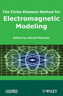
The Finite Element Method for Electromagnetic Modeling
ISTE Ltd and John Wiley & Sons Inc (Verlag)
978-1-84821-030-1 (ISBN)
- Titel z.Zt. nicht lieferbar
- Versandkostenfrei innerhalb Deutschlands
- Auch auf Rechnung
- Verfügbarkeit in der Filiale vor Ort prüfen
- Artikel merken
Chapters 1 to 4 present general 2D and 3D static and dynamic formulations by the use of scalar and vector unknowns and adapted interpolations for the fields (nodal, edge, face or volume).
Chapter 5 is dedicated to the presentation of different macroscopic behavior laws of materials and their implementation in a finite element context: anisotropy and hysteretic properties for magnetic sheets, iron losses, non-linear permanent magnets and superconductors.
More specific formulations are then proposed: the modeling of thin regions when finite elements become misfit (Chapter 6), infinite domains by using geometrical transformations (Chapter 7), the coupling of 2D and 3D formulations with circuit equations (Chapter 8), taking into account the movement, particularly in the presence of Eddy currents (Chapter 9) and an original approach for the treatment of geometrical symmetries when the sources are not symmetric (Chapter 10).
Chapters 11 to 13 are devoted to coupled problems: magneto-thermal coupling for induction heating, magneto-mechanical coupling by introducing the notion of strong and weak coupling and magneto-hydrodynamical coupling focusing on electromagnetic instabilities in fluid conductors.
Chapter 14 presents different meshing methods in the context of electromagnetism (presence of air) and introduces self-adaptive mesh refinement procedures. Optimization techniques are then covered in Chapter 15, with the adaptation of deterministic and probabilistic methods to the numerical finite element environment.
Chapter 16 presents a variational approach of electromagnetism, showing how Maxwell equations are derived from thermodynamic principles.
Gérard Meunier is the author of The Finite Element Method for Electromagnetic Modeling, published by Wiley.
Chapter 1. Introduction to Nodal Finite Elements. 1
Jean-Louis COULOMB
1.1. Introduction 1
1.1.1. The finite element method 1
1.2. The 1D finite element method 2
1.2.1. A simple electrostatics problem 2
1.2.2. Differential approach 3
1.2.3. Variational approach 4
1.2.4. First-order finite elements 6
1.2.5. Second-order finite elements 9
1.3. The finite element method in two dimensions 10
1.3.1. The problem of the condenser with square section 10
1.3.2. Differential approach 12
1.3.3. Variational approach 14
1.3.4. Meshing in first-order triangular finite elements 15
1.3.5. Finite element interpolation 17
1.3.6. Construction of the system of equations by the Ritz method 19
1.3.7. Calculation of the matrix coefficients 21
1.3.8. Analysis of the results 25
1.3.9. Dual formations, framing and convergence 42
1.3.10. Resolution of the nonlinear problems 44
1.3.11. Alternative to the variational method: the weighted residues method 45
1.4. The reference elements 47
1.4.1. Linear reference elements 48
1.4.2. Surface reference elements 49
1.4.3. Volume reference elements 52
1.4.4. Properties of the shape functions 53
1.4.5. Transformation from reference coordinates to domain coordinates 54
1.4.6. Approximation of the physical variable 56
1.4.7. Numerical integrations on the reference elements 60
1.4.8. Local Jacobian derivative method 63
1.5. Conclusion 66
1.6. References 66
Chapter 2. Static Formulations: Electrostatic, Electrokinetic, Magnetostatics 69
Patrick DULAR and Francis PIRIOU
2.1. Problems to solve 70
2.1.1. Maxwell’s equations 70
2.1.2. Behavior laws of materials 71
2.1.3. Boundary conditions 71
2.1.4. Complete static models 74
2.1.5. The formulations in potentials 75
2.2. Function spaces in the fields and weak formulations 82
2.2.1. Integral expressions: introduction 82
2.2.2. Definitions of function spaces 82
2.2.3. Tonti diagram: synthesis scheme of a problem 84
2.2.4. Weak formulations 86
2.3. Discretization of function spaces and weak formulations 91
2.3.1. Finite elements 91
2.3.2. Sequence of discrete spaces 93
2.3.3. Gauge conditions and source terms in discrete spaces 106
2.3.4. Weak discrete formulations 109
2.3.5. Expression of global variables 114
2.4. References 115
Chapter 3. Magnetodynamic Formulations 117
Zhuoxiang REN and Frédéric BOUILLAULT
3.1. Introduction 117
3.2. Electric formulations 119
3.2.1. Formulation in electric field 119
3.2.2. Formulation in combined potentials a - 120
3.2.3. Comparison of the formulations in field and in combined potentials 121
3.3. Magnetic formulations 123
3.3.1. Formulation in magnetic field 123
3.3.2. Formulation in combined potentials t - ɸ 124
3.3.3. Numerical example 125
3.4. Hybrid formulation 127
3.5. Electric and magnetic formulation complementarities 128
3.5.1. Complementary features 128
3.5.2. Concerning the energy bounds 129
3.5.3. Numerical example 129
3.6. Conclusion 133
3.7. References 134
Chapter 4. Mixed Finite Element Methods in Electromagnetism 139
Bernard BANDELIER and Françoise RIOUX-DAMIDAU
4.1. Introduction 139
4.2. Mixed formulations in magnetostatics 140
4.2.1. Magnetic induction oriented formulation 141
4.2.2. Formulation oriented magnetic field 144
4.2.3. Formulation in induction and field 146
4.2.4. Alternate case 147
4.3. Energy approach: minimization problems, searching for a saddle-point 147
4.3.1. Minimization of a functional calculus related to energy 147
4.3.2. Variational principle of magnetic energy 149
4.3.3. Searching for a saddle-point 151
4.3.4. Functional calculus related to the constitutive relationship 154
4.4. Hybrid formulations 154
4.4.1. Magnetic induction oriented hybrid formulation 154
4.4.2. Hybrid formulation oriented magnetic field 156
4.4.3. Mixed hybrid method 157
4.5. Compatibility of approximation spaces – inf-sup condition 157
4.5.1. Mixed magnetic induction oriented formulation 158
4.5.2. Mixed formulation oriented magnetic field 160
4.5.3. General case 160
4.6. Mixed finite elements, Whitney elements 161
4.6.1. Magnetic induction oriented formulation 162
4.6.2. Magnetic field oriented formulation 163
4.7. Mixed formulations in magnetodynamics 164
4.7.1. Magnetic field oriented formulation 164
4.7.2. Formulation oriented electric field 167
4.8. Solving techniques 167
4.8.1. Penalization methods 168
4.8.2. Algorithm using the Schur complement 171
4.9. References 174
Chapter 5. Behavior Laws of Materials 177
Frédéric BOUILLAULT, Afef KEDOUS-LEBOUC, Gérard MEUNIER, Florence OSSART and Francis PIRIOU
5.1. Introduction 177
5.2. Behavior law of ferromagnetic materials 178
5.2.1. Definitions 178
5.2.2. Hysteresis and anisotropy 179
5.2.3. Classificiation of models dealing with the behavior law 180
5.3. Implementation of nonlinear behavior models 183
5.3.1. Newton method 183
5.3.2. Fixed point method 187
5.3.3. Particular case of a behavior with hysteresis 191
5.4. Modeling of magnetic sheets 192
5.4.1. Some words about magnetic sheets 192
5.4.2. Example of stress in the electric machines 192
5.4.3. Anisotropy of sheets with oriented grains 194
5.4.4. Hysteresis and dynamic behavior under uniaxial stress 200
5.4.5. Determination of iron losses in electric machines: nonlinear isotropic finite element modeling and calculation of the losses a posteriori 209
5.4.6. Conclusion 215
5.5. Modeling of permanent magnets 216
5.5.1. Introduction. 216
5.5.2. Magnets obtained by powder metallurgy 216
5.5.3. Study of linear anisotropic behavior 218
5.5.4. Study of nonlinear behavior 220
5.5.5. Implementation of the model in finite element software 223
5.5.6. Validation: the experiment by Joel Chavanne 224
5.5.7. Conductive magnet subjected to an AC field 225
5.6. Modeling of superconductors 226
5.6.1. Introduction 226
5.6.2. Behavior of superconductors 227
5.6.3. Modeling of electric behavior of superconductors 230
5.6.4. Particular case of the Bean model 232
5.6.5. Examples of modeling 237
5.7. Conclusion 240
5.8. References 241
Chapter 6. Modeling on Thin and Line Regions 245
Christophe GUÉRIN
6.1. Introduction 245
6.2. Different special elements and their interest 245
6.3. Method for taking into account thin regions without potential jump 249
6.4. Method for taking into account thin regions with potential jump 250
6.4.1. Analytical integration method 251
6.4.2. Numerical integration method 252
6.5. Method for taking thin regions into account 255
6.6. Thin and line regions in magnetostatics 256
6.6.1. Thin and line regions in magnetic scalar potential formulations 256
6.6.2. Thin and line regions in magnetic vector potential formulations 257
6.7. Thin and line regions in magnetoharmonics 257
6.7.1. Solid conducting regions presenting a strong skin effect 258
6.7.2. Thin conducting regions 265
6.8. Thin regions in electrostatic problems: “electric harmonic problems” and electric conduction problems 272
6.9. Thin thermal regions 272
6.10. References 273
Chapter 7. Coupling with Circuit Equations 277
Gérard MEUNIER, Yvan LEFEVRE, Patrick LOMBARD and Yann LE FLOCH
7.1. Introduction 277
7.2. Review of the various methods of setting up electric circuit equations 278
7.2.1. Circuit equations with nodal potentials 278
7.2.2. Circuit equations with mesh currents 279
7.2.3. Circuit equations with time integrated nodal potentials 280
7.2.4. Formulation of circuit equations in the form of state equations 281
7.2.5. Conclusion on the methods of setting up electric equations 283
7.3. Different types of coupling 284
7.3.1. Indirect coupling 285
7.3.2. Integro-differential formulation 285
7.3.3. Simultaneous resolution 285
7.3.4. Conclusion 285
7.4. Establishment of the “current-voltage” relations 286
7.4.1. Insulated massive conductor with two ends: basic assumptions and preliminary relations 286
7.4.2. Current-voltage relations using the magnetic vector potential 287
7.4.3. Current-voltage relations using magnetic induction 288
7.4.4. Wound conductors 290
7.4.5. Losses in the wound conductors 291
7.5. Establishment of the coupled field and circuit equations 292
7.5.1. Coupling with a vector potential formulation in 2D 292
7.5.2. Coupling with a vector potential formulation in 3D 303
7.5.3. Coupling with a scalar potential formulation in 3D 310
7.6. General conclusion 317
7.7. References 318
Chapter 8. Modeling of Motion: Accounting for Movement in the Modeling of Magnetic Phenomena 321
Vincent LECONTE
8.1. Introduction 321
8.2. Formulation of an electromagnetic problem with motion 322
8.2.1. Definition of motion 322
8.2.2. Maxwell equations and motion 325
8.2.3. Formulations in potentials 329
8.2.4. Eulerian approach 335
8.2.5. Lagrangian approach 338
8.2.6. Example application 342
8.3. Methods for taking the movement into account 346
8.3.1. Introduction. 346
8.3.2. Methods for rotating machines 346
8.3.3. Coupling methods without meshing and with the finite element method 348
8.3.4. Coupling of boundary integrals with the finite element method 350
8.3.5. Automatic remeshing methods for large distortions 355
8.4. Conclusion 362
8.5. References 363
Chapter 9. Symmetric Components and Numerical Modeling 369
Jacques LOBRY, Eric NENS and Christian BROCHE
9.1. Introduction 369
9.2. Representation of group theory 371
9.2.1. Finite groups 371
9.2.2. Symmetric functions and irreducible representations 374
9.2.3. Orthogonal decomposition of a function 378
9.2.4. Symmetries and vector fields 379
9.3. Poisson’s problem and geometric symmetries 384
9.3.1. Differential and integral formulations 384
9.3.2. Numerical processing 387
9.4. Applications 388
9.4.1. 2D magnetostatics 388
9.4.2. 3D magnetodynamics 394
9.5. Conclusions and future work 403
9.6. References 404
Chapter 10. Magneto-thermal Coupling 405
Mouloud FÉLIACHI and Javad FOULADGAR
10.1. Introduction 405
10.2. Magneto-thermal phenomena and fundamental equations 406
10.2.1. Electromagentism 406
10.2.2. Thermal 408
10.2.3. Flow 408
10.3. Behavior laws and couplings 409
10.3.1. Electrmagnetic phenomena 409
10.3.2. Thermal phenomena 409
10.3.3. Flow phenomena 409
10.4. Resolution methods 409
10.4.1. Numerical methods 409
10.4.2. Semi-analytical methods 410
10.4.3. Analytical-numerical methods 411
10.4.4. Magneto-thermal coupling models 411
10.5. Heating of a moving work piece 413
10.6. Induction plasma 417
10.6.1. Introduction 417
10.6.2. Inductive plasma installation 418
10.6.3. Mathematical models 418
10.6.4. Results 426
10.6.5. Conclusion 427
10.7. References 428
Chapter 11. Magneto-mechanical Modeling 431
Yvan LEFEVRE and Gilbert REYNE
11.1. Introduction 431
11.2. Modeling of coupled magneto-mechancial phenomena 432
11.2.1. Modeling of mechanical structure 433
11.2.2. Coupled magneto-mechanical modeling 437
11.2.3. Conclusion 442
11.3. Numerical modeling of electromechancial conversion in conventional actuators 442
11.3.1. General simulation procedure 443
11.3.2. Global magnetic force calculation method 444
11.3.3. Conclusion 447
11.4. Numerical modeling of electromagnetic vibrations 447
11.4.1. Magnetostriction vs. magnetic forces 447
11.4.2. Procedure for simulating vibrations of magnetic origin 449
11.4.3. Magnetic forces density 449
11.4.4. Case of rotating machine teeth 452
11.4.5. Magnetic response modeling 453
11.4.6. Model superposition method 455
11.4.7. Conclusion 458
11.5. Modeling strongly coupled phenomena 459
11.5.1. Weak coupling and strong coupling from a physical viewpoint 459
11.5.2. Weak coupling or strong coupling problem from a numerical modeling analysis 460
11.5.3. Weak coupling and intelligent use of software tools 461
11.5.4. Displacement and deformation of a magnetic system 463
11.5.5. Structural modeling based on magnetostrictive materials 465
11.5.6. Electromagnetic induction launchers 469
11.6. Conclusion 470
11.7. References 471
Chapter 12. Magnetohydrodynamics: Modeling of a Kinematic Dynamo 477
Franck PLUNIAN and Philippe MASSÉ
12.1. Introduction 477
12.1.1. Generalities 477
12.1.2. Maxwell’s equations and Ohm’s law 481
12.1.3. The induction equation 482
12.1.4. The dimensionless equation 483
12.2. Modeling the induction equation using finite elements 485
12.2.1. Potential (A,ɸ) quadric-vector formulation 485
12.2.2. 2D1/2 quadri-vector potential formulation 488
12.3. Some simulation examples 491
12.3.1. Screw dynamo (Ponomarenko dynamo) 491
12.3.2. Two-scale dynamo without walls (Roberts dynamo) 495
12.3.3. Two-scale dynamo with walls 498
12.3.4. A dynamo at the industrial scale 502
12.4. Modeling of the dynamic problem 503
12.5. References 504
Chapter 13. Mesh Generation 509
Yves DU TERRAIL COUVAT, François-Xavier ZGAINSKI and Yves MARÉCHAL
13.1. Introduction 509
13.2. General definition 510
13.3. A short history 512
13.4. Mesh algorithms 512
13.4.1. The basic algorithms 512
13.4.2. General mesh algorithms 518
13.5. Mesh regularization 526
13.5.1. Regularization by displacement of nodes 526
13.5.2. Regularization by bubbles 528
13.5.3. Adaptation of nodes population 530
13.5.4. Insertion in meshing algorithms 530
13.5.5. Value of bubble regularization 531
13.6. Mesh processer and modeling environment 533
13.6.1. Some typical criteria 533
13.6.2. Electromagnetism and meshing constraints 534
13.7. Conclusion 541
13.8. References 541
Chapter 14. Optimization 547
Jean-Louis COULOMB
14.1. Introduction 547
14.1.1. Optimization: who, why, how? 547
14.1.2. Optimization by numerical simulation: is this reasonable? 548
14.1.3. Optimization by numerical simulation: difficulties 549
14.1.4. Numerical design of experiments (DOE) method: an elegant solution 549
14.1.5. Sensitivity analysis: an “added value” accessible by simulation 550
14.1.6. Organization of this chapter 551
14.2. Optimization methods 551
14.2.1. Optimization problems: some definitions 551
14.2.2. Optimization problems without constraints 553
14.2.3. Constrained optimization problems 559
14.2.4. Multi-objective optimization 560
14.3. Design of experiments (DOE) method 562
14.3.1. The direct control of the simulation tool by an optimization algorithm: principle and disadvantages 562
14.3.2. The response surface: an approximation enabling indirect optimization 563
14.3.3. DOE method: a short history 565
14.3.4. DOE method: a simple example 565
14.4. Response surfaces 572
14.4.1. Basic principles 572
14.4.2. Polynomial surfaces of degree 1 without interaction: simple but sometimes useful 573
14.4.3. Polynomial surfaces of degree 1 with interactions: quite useful for screening 573
14.4.4. Polynomial surfaces of degree 2: a first approach for nonlinearities 574
14.4.5. Response surfaces of degrees 1 and 2: interests and limits 576
14.4.6. Response surfaces by combination of radial functions 576
14.4.7. Response surfaces using diffuse elements 577
14.4.8. Adaptive response surfaces 579
14.5. Sensitivity analysis 579
14.5.1. Finite difference method 579
14.5.2. Method for local derivation of the Jacobian matrix 580
14.5.3. Steadiness of state variables: steadiness of state equations 581
14.5.4. Sensitivity of the objective function: the adjoint state method 583
14.5.5. Higher order derivative 583
14.6. A complete example of optimization 584
14.6.1. The problem of optimization 584
14.6.2. Determination of the influential parameters by the DOE method 585
14.6.3. Approximation of the objective function by a response surface 587
14.6.4. Search for the optimum on the response surface 587
14.6.5. Verification of the solution by simulation 587
14.7. Conclusion 588
14.8. References 588
List of Authors 595
Index 599
| Erscheint lt. Verlag | 24.10.2008 |
|---|---|
| Verlagsort | London |
| Sprache | englisch |
| Maße | 155 x 236 mm |
| Gewicht | 1066 g |
| Themenwelt | Naturwissenschaften ► Physik / Astronomie ► Elektrodynamik |
| ISBN-10 | 1-84821-030-2 / 1848210302 |
| ISBN-13 | 978-1-84821-030-1 / 9781848210301 |
| Zustand | Neuware |
| Haben Sie eine Frage zum Produkt? |
aus dem Bereich


