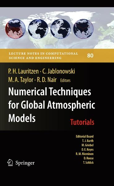
Numerical Techniques for Global Atmospheric Models (eBook)
XVI, 564 Seiten
Springer Berlin (Verlag)
978-3-642-11640-7 (ISBN)
This book surveys recent developments in numerical techniques for global atmospheric models. It is based upon a collection of lectures prepared by leading experts in the field. The chapters reveal the multitude of steps that determine the global atmospheric model design. They encompass the choice of the equation set, computational grids on the sphere, horizontal and vertical discretizations, time integration methods, filtering and diffusion mechanisms, conservation properties, tracer transport, and considerations for designing models for massively parallel computers. A reader interested in applied numerical methods but also the many facets of atmospheric modeling should find this book of particular relevance.
Foreword
6
Preface
8
Contents
14
Contributors
16
Part I Equations of Motion and Basic Ideas on Discretizations 18
Chapter 1: Some Basic Dynamics Relevant to the Design of Atmospheric Model Dynamical Cores 19
1.1 Introduction 19
1.2 The Multiscale Nature of Atmospheric Dynamics 20
1.3 Governing Equations 21
1.3.1 Approximate Equation Sets 23
1.4 Fast Waves 25
1.4.1 Acoustic Waves 25
1.4.2 Inertio-Gravity Waves 26
1.4.3 Phase Velocity and Group Velocity 28
1.5 Balance 30
1.5.1 Hydrostatic Balance 30
1.5.2 Geostrophic Balance 31
1.5.3 Conditions for Hydrostatic Balance to be a Good Approximation 31
1.5.4 Balance and Nonlocality 32
1.6 Sketch of Quasigeostrophic Theory 33
1.6.1 Rossby Waves 35
1.7 Eulerian and Lagrangian Timescales 36
1.8 Turbulence and Cascades 37
1.8.1 Three Dimensional Turbulence 37
1.8.2 Two-dimensional Turbulence 38
1.8.3 Energy Upscale, Enstrophy Downscale 39
1.8.4 Application to the Real Atmosphere 41
1.9 Conclusion 42
References 42
Chapter 2: Waves, Hyperbolicity and Characteristics 44
2.1 Introduction 44
2.2 The Method of Characteristics 45
2.3 The Normal Modes of the Hydrostatic Equations 47
2.4 The Modes of the Primitive Equations on the Sphere 52
2.5 Discussion and Conclusions 56
References 57
Chapter 3: Horizontal Discretizations: Some Basic Ideas 58
3.1 Introduction 58
3.2 Wave Propagation and Staggered Grids 58
3.2.1 Gravity Waves in One-Dimension 59
3.2.2 Inertio-Gravity Waves in Two-Dimensions 63
3.2.3 Rossby Wave Propagation on the C-grid 67
3.3 Conservation Properties 68
3.3.1 Energy Conservation: Coriolis Terms 69
3.3.2 Energy Conservation: Pressure Gradient Terms 71
3.4 Conclusions 71
References 72
Chapter 4: Vertical Discretizations: Some Basic Ideas 73
4.1 Introduction 73
4.2 Alternative Vertical Coordinates 73
4.2.1 Examples 74
4.3 Bottom and Top Boundary Conditions 75
4.4 The Simmons and Burridge Energy and Angular Momentum Conserving Scheme 77
4.4.1 Hydrostatic Equation 77
4.4.2 Angular Momentum Conservation 78
4.4.3 Energy Conservation 79
4.5 Wave Dispersion and Balance 80
4.5.1 The Lorenz and Charney–Phillips Grids 80
4.5.2 Lorenz Grid Computational Mode 81
4.5.3 Compressible Euler Equations 81
4.5.3.1 Acoustic Waves 82
4.5.3.2 Inertio-Gravity Waves 83
4.5.3.3 Rossby Waves 83
4.5.3.4 Numerical Dispersion Relations for Some Example Configurations 83
4.6 Conclusion 87
References 87
Chapter 5: Time Discretization: Some Basic Approaches 89
5.1 Introduction 89
5.2 Stability, Consistency and Convergence 91
5.2.1 Truncation Error 91
5.2.2 Convergence 93
5.2.3 Stability 94
5.3 Additional Measures of Stability and Accuracy 95
5.3.1 A-Stability 95
5.3.2 Phase-Speed Errors 96
5.3.3 Single-Stage, Single-Step Schemes 98
5.3.4 Application to PDEs 101
5.3.5 L-Stability 102
5.4 Runge–Kutta (Multi-Stage) Methods 103
5.4.1 Explicit Two-Stage Schemes 104
5.4.2 Explicit Three- and Four-Stage Schemes 107
5.4.3 Strong-Stability Preserving Methods 110
5.4.4 Diagonally Implicit Runge–Kutta Methods 111
5.5 Multistep Methods 112
5.5.1 Explicit Two-Step Schemes 112
5.5.2 The Leapfrog Scheme 113
5.5.3 The Two-Step Adams–Bashforth Scheme 115
5.6 Summary Discussion 117
References 117
Chapter 6: Stabilizing Fast Waves 119
6.1 Introduction 119
6.2 The Projection Method 121
6.2.1 Forward-in-Time Implementation 122
6.2.2 Leapfrog Implementation 124
6.2.3 Solving the Poisson Equation for Pressure 125
6.3 The Semi-Implicit Method 126
6.3.1 Large Time Steps and Poor Accuracy 127
6.3.2 A Prototype Problem 129
6.3.3 Semi-Implicit Solution of the Shallow-Water Equations 131
6.3.4 Semi-implicit Solution of the Compressible Governing Equations 132
6.3.5 Numerical Implementation 137
6.4 Fractional-Step Methods 138
6.4.1 Complete Operator Splitting 138
6.4.2 Partially-Split Operators 144
6.5 Summary Discussion 151
References 153
Part II Conservation Laws, Finite-Volume Methods, Remapping Techniques and Spherical Grids 155
Chapter 7: Momentum, Vorticity and Transport: Considerations in the Design of a Finite-Volume Dynamical Core 156
7.1 Introduction 156
7.2 Reference Frames and Conceptual Constructs 158
7.3 Evolution Equations from a Lagrangian Perspective 161
7.3.1 The Reynolds Transport Theorem 162
7.3.2 Conservation of Mass and Tracer Substance 164
7.3.3 A Statement of Newton's Second Law 166
7.3.4 Dynamics of Vorticity 168
7.3.4.1 Conservation of Circulation 171
7.3.4.2 Conservation of Absolute Vorticity 174
7.3.5 Summary of Evolution Equations 174
7.4 The Various Flavors of F = m a 175
7.4.1 The Advective Form 175
7.4.2 The Flux Form 178
7.4.3 The Vector-Invariant Form 179
7.4.4 The Vorticity-Divergence Form 180
7.5 The Process of Discretization 181
7.5.1 Target Application: Joint Climate-Weather Prediction 182
7.5.2 Grid Staggering: C-grid Staggering 183
7.5.3 Mesh: Locally-Orthogonal Meshes 183
7.5.4 Form of Momentum Equation: The Vector-Invariant Form 184
7.6 Building a Discrete Model 184
7.6.1 Defining the Mesh and Location of Variables 184
7.6.2 Continuous Prognostic Equation 185
7.6.3 Discrete Prognostic Equation 186
7.6.4 Derived Equation 187
7.7 Constraining the Evolution of Velocity Through the Transport of Absolute Vorticity 191
7.7.1 Considerations when Specifying . 192
7.7.2 Considerations when Specifying T 193
7.8 Final Thoughts 194
References 195
Chapter 8: Atmospheric Transport Schemes: Desirable Properties and a Semi-Lagrangian View on Finite-Volume Discretizations 197
8.1 Introduction 197
8.2 The Continuous Equation 199
8.2.1 Representation of Mass in Atmospheric Models 199
8.2.2 Consistency in the Mass Equations 201
8.3 Desirable Properties 202
8.3.1 Accuracy (Error Norms) 203
8.3.1.1 Linear Test Cases 203
8.3.1.2 Non-Linear Test Cases 206
8.3.2 Conservation of Mass 209
8.3.3 Optimal Diffusion and Dispersion Properties 210
8.3.4 Tracer and Air Mass Consistency 211
8.3.5 Divergence Preservation 211
8.3.6 Physical Realizability (Monotone, Positive-Definite, Non-Oscillatory, Shape-Preserving) 212
8.3.7 Preservation of Pre-Existing Functional Relations Between Species (Correlations) 212
8.3.8 Robustness 215
8.3.9 Parallel Computational Efficiency 215
8.3.10 Multi-Tracer Efficiency 215
8.3.11 Geometric Flexibility 216
8.4 Problem Formulation: Discrete Schemes 216
8.4.1 (Semi-)Lagrangian Schemes 217
8.4.2 Eulerian Scheme 221
8.4.3 Equivalence Between the Lagrangian and Eulerian Discretizations 223
8.5 Discrete Schemes: Approximations 224
8.5.1 Approximation to Areas 225
8.5.1.1 Lagrangian Area Approximations 225
8.5.1.2 Eulerian Flux Area Approximations 227
8.5.1.3 Comment on Area Approximations 230
8.5.2 Sub-Grid-Scale Reconstruction 232
8.5.2.1 One-Dimensional Reconstruction Functions 232
8.5.2.2 Two-Dimensional Reconstruction Functions 244
8.5.3 Practical Integration Over Areas 247
8.5.3.1 Direct Integration Using Gaussian Quadrature 248
8.5.3.2 Converting Area-integrals into Line-integrals 249
8.5.3.3 Extension to Spherical Geometry 251
8.6 Extension to Three Dimensions 252
8.6.1 Floating Lagrangian Vertical Coordinate 252
8.6.2 Operator Splitting 253
8.6.3 Rigorous Three-dimensional Approach 254
8.7 Time-integration and Tracer Transport 254
8.7.1 Different Schemes Air and Tracers 254
8.7.2 Different Time-steps for Air and Tracers (Sub-Cycling, Super-Cycling) 254
8.7.3 Semi-Implicit Time-Stepping for Air and Explicit for Tracers 257
8.8 Final Remarks 257
References 258
Chapter 9: Emerging Numerical Methods for Atmospheric Modeling 263
9.1 Introduction 263
9.2 The DG Method 265
9.2.1 Conservation Laws 266
9.2.2 The DG Method for 1D Problems 266
9.2.3 Galerkin Formulation 267
9.2.4 Space Discretization 268
9.2.4.1 Modal Formulation 269
9.2.4.2 Nodal Formulation 274
9.2.5 Time Integration 276
9.2.6 DG 1D Computational Examples 278
9.3 DG for 2D Cartesian Problems 280
9.3.1 Space Discretization 282
9.3.1.1 2D Modal Form 283
9.3.1.2 2D Nodal Form 284
9.3.1.3 Approximating the Integrals 285
9.3.2 Computational Examples: Advection Tests 287
9.3.2.1 Solid-Body Rotation Test 287
9.3.2.2 Deformational Flow Test 289
9.3.2.3 Barotropic Vorticity Equation 290
9.4 Limiters for DG Methods 293
9.4.1 The 1D Limiters for DG Methods 294
9.4.1.1 The Minmod Limiter 294
9.4.1.2 Generalized Slope Limiter 296
9.4.1.3 The Moment Limiter 297
9.4.1.4 The WENO-Based Limiter 298
9.4.1.5 Computational Examples with Limiters 298
9.4.2 2D Limiters for the DG Method 301
9.4.2.1 A Limiter for the DG P2 Method 301
9.4.2.2 A Positivity-Preserving Slope Limiter 302
9.4.2.3 2D Numerical Experiments 304
9.5 The DG Methods on the Sphere 305
9.5.1 The Shallow Water Model on the Sphere 306
9.5.2 The Cubed-Sphere Geometry 307
9.5.3 The Shallow Water Model on the Cubed-Sphere 308
9.5.4 The Computational Domain 309
9.5.5 The DG Discretization of the SW Equations 310
9.5.5.1 Flux Exchanges at the Cubed-Sphere Edges 312
9.5.5.2 Numerical Integration of the SW Model 312
9.5.6 Numerical Experiments 313
9.5.6.1 Advection Test 313
9.5.6.2 Deformational Flow Test 314
9.5.6.3 Solid-Body Rotation Test 316
9.5.6.4 Barotropic Instability Test 316
9.6 Concluding Remarks 318
References 319
Chapter 10: Voronoi Tessellations and Their Application to Climate and Global Modeling 324
10.1 Introduction 324
10.2 Voronoi and Delaunay Tessellations 329
10.2.1 Definitions and Properties 329
10.2.2 Construction Algorithms 330
10.3 Centroidal Voronoi Tessellations 333
10.3.1 Definitions and Properties 334
10.3.1.1 Centroidal Voronoi Tessellations of Surfaces 336
10.3.2 Algorithms for Constructing CVTs 337
10.3.3 The Relation Between the Density Function and the Local Mesh Size 340
10.4 Application to Climate and Global Modeling 341
10.4.1 Global SCVT Meshes 341
10.4.1.1 Uniform SCVT Meshes vs. Icosahedral-Bisection Meshes 342
10.4.1.2 Locally Refined SCVT Meshes 342
10.4.1.3 Nested SCVT Meshes 345
10.4.2 CVT-Based Regional Meshes of the North Atlantic Ocean 347
10.4.3 Numerical Simulations with SCVT Meshes 348
10.4.3.1 Mesh Decomposition for Parallel Computing 348
10.4.3.2 Example Numerical Methods 349
10.5 Summary 349
References 350
Part III Practical Considerations for Dynamical Cores in Weather and Climate Models 354
Chapter 11: Conservation in Dynamical Cores: What, How and Why? 355
11.1 Introduction 355
11.2 Conservation Properties of the Continuous Adiabatic Frictionless Governing Equations 356
11.2.1 Flux-Form Conservation Laws 356
11.2.2 Lagrangian Conservation Laws 356
11.2.3 Conserved Integrals 357
11.2.4 Kinematic Identities 357
11.3 What Conservation Properties can we Obtain in Numerical Models? 358
11.4 Which Conservation Properties are the Most Relevant or Important? 360
11.4.1 Finite Resolution Effects 360
11.4.2 The Adiabatic Frictionless Limit 361
11.4.3 Energy 362
11.4.4 Spurious Sources vs Physical Sources 363
11.5 Conclusion 365
References 365
Chapter 12: Conservation of Mass and Energy for the Moist Atmospheric Primitive Equations on Unstructured Grids 366
12.1 Introduction 366
12.2 Quadrilateral Tilings of the Sphere 369
12.3 Continuum Formulation of the Equations 371
12.4 Discrete Formulation of the Equations 374
12.4.1 Consistency 376
12.4.2 Discrete Global Integral 377
12.4.3 Compatibility Identities 377
12.4.4 Discrete Conservation of Mass and Tracer Mass 378
12.4.5 Discrete Conservation of Energy 379
12.4.6 Potential Temperature Formulation 381
12.5 Example Computations 381
12.5.1 Adiabatic Results 383
12.5.2 Non-Adiabatic Results 384
12.6 Conclusions 386
References 387
Chapter 13: The Pros and Cons of Diffusion, Filters and Fixers in Atmospheric General Circulation Models 390
13.1 Introduction 390
13.1.1 Model Equations and the Representation of Explicit Diffusion 393
13.1.2 Overview of the Chapter 394
13.2 Selected Dynamical Cores and Test Cases 394
13.3 Explicit Horizontal Diffusion 395
13.3.1 Generic Form of the Explicit Diffusion Mechanism 396
13.3.2 Particular Forms of Explicit Diffusion in GCMs 396
13.3.3 Practical Considerations: Linear High-Order Diffusion Operators 401
13.3.4 Choice of the Diffusion Coefficient: Damping Time Scales 402
13.3.4.1 Diffusion Coefficients in Spectral Transform Models 404
13.3.4.2 The Concept of Spectral Viscosity 407
13.3.4.3 Diffusion Coefficients in Grid-Point Models 409
13.3.4.4 Examples of Diffusion Coefficients in Spectral Models 410
13.3.4.5 Examples of Diffusion Coefficients in Grid Point Models 413
13.3.4.6 Caveats 414
13.3.5 Choice of the Diffusion Coefficient: Stability 414
13.3.6 Nonlinear Horizontal Diffusion 416
13.3.7 Physical Consistency 418
13.3.8 Diffusion Properties in Practice: The Model CAM 3.1 420
13.4 Divergence and Vorticity Damping, External Mode Damping and Sponge Layers 425
13.4.1 2D Divergence Damping 425
13.4.1.1 Selection of the 2D Divergence Damping Coefficient 427
13.4.1.2 Example: The Effects of Divergence Damping 428
13.4.1.3 2D Divergence Damping: Avoiding Confusion 431
13.4.2 3D Divergence Damping (or Acoustic Mode Filtering) 433
13.4.3 Vorticity Damping 434
13.4.4 External Mode Damping 435
13.4.5 Sponge Layer Mechanisms at the Model Top 436
13.4.5.1 Rayleigh Friction 437
13.4.5.2 Diffusive Sponges 441
13.4.5.3 Vertical Velocity Damping 442
13.4.5.4 Courant Number Limiter 443
13.5 Explicit Filtering Techniques 444
13.5.1 Time Filters 445
13.5.1.1 Robert-Asselin Filter 445
13.5.1.2 Time Filter for Extrapolated Values 447
13.5.2 Spatial Filters 448
13.5.2.1 Digital Grid Point Filters 448
13.5.2.2 Examples: Applications of the Shapiro Filter 451
13.5.2.3 Spectral Filters: Fourier Filtering 453
13.5.2.4 Local Spectral Filters 455
13.6 Inherent Numerical Damping 456
13.6.1 Order of the Numerical Scheme 457
13.6.2 Monotonicity Constraints and Shape Preservation 461
13.6.3 Decentering Mechanisms 463
13.6.3.1 Decentering in Semi-implicit Semi-Lagrangian Models 464
13.6.3.2 Forward-Biasing of Trapezoidal Time Integrations 466
13.6.4 Damping by Semi-Lagrangian Interpolation 467
13.7 Fixers and Thoughts About Conservation Properties 472
13.7.1 Dry Air Mass Fixer 473
13.7.2 Filling Algorithms for Tracers 478
13.7.2.1 Local Filling Algorithms 479
13.7.2.2 Global Filling Algorithms 480
13.7.3 Total Energy Fixers 480
13.7.3.1 Different Forms of the Total Energy Equation 482
13.7.3.2 Ad Hoc Corrections of Total Energy 485
13.8 Final Thoughts 487
Appendix: Overview of Selected Dynamical Cores 489
References 491
Chapter 14: Kinetic Energy Spectra and Model Filters 503
14.1 Introduction 503
14.2 Kinetic Energy Spectra and Atmospheric Dynamics 505
14.3 Model Dissipation and Spectral Damping 507
14.4 Grid Staggering and Spatial Discretizations 510
14.5 Semi-Implicit Semi-Lagrangian Formulations 513
14.6 Conclusions 517
References 518
Chapter 15: A Perspective on the Role of the Dynamical Core in the Development of Weather and Climate Models 521
15.1 Introduction 521
15.2 Definition and Description of the Model 522
15.3 Construction of Weather and Climate Models 525
15.4 Analysis of the Atmospheric Equations of Motion 529
15.5 Numerical Expression of the Atmospheric Equations of Motion 532
15.6 Synthesis and Future Directions 535
15.6.1 Model-Relevant Principles 536
15.6.2 Lessons Learned about Dynamical Cores 536
15.6.2.1 Consistency 536
15.6.2.2 Locality 537
15.6.2.3 Horizontal Advection 537
15.6.2.4 Vertical Velocity 537
15.6.2.5 Mixing, Filters and Fixers 537
15.6.3 Future Directions 538
15.6.3.1 Divergence 538
15.6.3.2 Mixing, Filters, and Fixers (Chap. 13) 539
15.6.3.3 Non-Hydrostatic 539
15.6.3.4 Grids 539
15.6.3.5 Coupling 540
15.7 Conclusions 540
References 542
16 Refactoring Scientific Applications for Massive Parallelism 546
16.1 Introduction 546
16.2 Background 549
16.3 Scalability 550
16.3.1 Scalability of Memory Usage 553
16.3.2 Replicated Metadata 553
16.3.3 Excessive Global-Sized Arrays 555
16.3.4 Serial I/O 555
16.4 Scalability of Execution Time 556
16.4.1 Non-scalable Initialization 557
16.4.2 Non-scalable Inter-processor Communication 557
16.5 Other Impediments 559
16.5.1 Debugging at Scale 559
16.5.2 Pre/Post Processing 560
16.6 Conclusions 561
References 562
Editorial Policy 564
Lecture Notesin Computational Scienceand Engineering 566
Monographs in Computational Scienceand Engineering 570
Texts in Computational Scienceand Engineering 570
| Erscheint lt. Verlag | 29.3.2011 |
|---|---|
| Reihe/Serie | Lecture Notes in Computational Science and Engineering | Lecture Notes in Computational Science and Engineering |
| Zusatzinfo | XVI, 564 p. |
| Verlagsort | Berlin |
| Sprache | englisch |
| Themenwelt | Mathematik / Informatik ► Mathematik ► Statistik |
| Mathematik / Informatik ► Mathematik ► Wahrscheinlichkeit / Kombinatorik | |
| Technik | |
| Schlagworte | atmospheric general circulation models • conservation laws • numerical methods for global modeling • Partial differential equations • spherical grids |
| ISBN-10 | 3-642-11640-X / 364211640X |
| ISBN-13 | 978-3-642-11640-7 / 9783642116407 |
| Haben Sie eine Frage zum Produkt? |
Größe: 15,8 MB
DRM: Digitales Wasserzeichen
Dieses eBook enthält ein digitales Wasserzeichen und ist damit für Sie personalisiert. Bei einer missbräuchlichen Weitergabe des eBooks an Dritte ist eine Rückverfolgung an die Quelle möglich.
Dateiformat: PDF (Portable Document Format)
Mit einem festen Seitenlayout eignet sich die PDF besonders für Fachbücher mit Spalten, Tabellen und Abbildungen. Eine PDF kann auf fast allen Geräten angezeigt werden, ist aber für kleine Displays (Smartphone, eReader) nur eingeschränkt geeignet.
Systemvoraussetzungen:
PC/Mac: Mit einem PC oder Mac können Sie dieses eBook lesen. Sie benötigen dafür einen PDF-Viewer - z.B. den Adobe Reader oder Adobe Digital Editions.
eReader: Dieses eBook kann mit (fast) allen eBook-Readern gelesen werden. Mit dem amazon-Kindle ist es aber nicht kompatibel.
Smartphone/Tablet: Egal ob Apple oder Android, dieses eBook können Sie lesen. Sie benötigen dafür einen PDF-Viewer - z.B. die kostenlose Adobe Digital Editions-App.
Buying eBooks from abroad
For tax law reasons we can sell eBooks just within Germany and Switzerland. Regrettably we cannot fulfill eBook-orders from other countries.
aus dem Bereich


