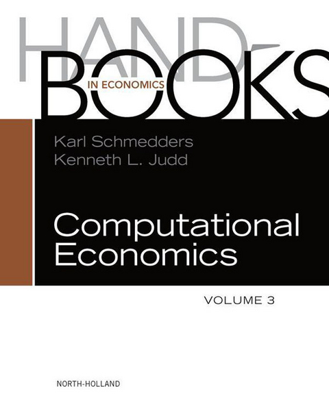
Handbook of Computational Economics summarizes recent advances in economic thought, revealing some of the potential offered by modern computational methods. With computational power increasing in hardware and algorithms, many economists are closing the gap between economic practice and the frontiers of computational mathematics. In their efforts to accelerate the incorporation of computational power into mainstream research, contributors to this volume update the improvements in algorithms that have sharpened econometric tools, solution methods for dynamic optimization and equilibrium models, and applications to public finance, macroeconomics, and auctions. They also cover the switch to massive parallelism in the creation of more powerful computers, with advances in the development of high-power and high-throughput computing. Much more can be done to expand the value of computational modeling in economics. In conjunction with volume one (1996) and volume two (2006), this volume offers a remarkable picture of the recent development of economics as a science as well as an exciting preview of its future potential. - Samples different styles and approaches, reflecting the breadth of computational economics as practiced today- Focuses on problems with few well-developed solutions in the literature of other disciplines- Emphasizes the potential for increasing the value of computational modeling in economics
Learning About Learning in Dynamic Economic Models*
David A. Kendricka, Hans M. Ammanb and Marco P. Tuccic, aDepartment of Economics, University of Texas, Austin, Texas 78712, USA, bUtrecht School of Economics, Utrecht University, Heidelberglaan, 8, Utrecht, 3584 CS, The Netherlands, cDipartimento di Economia Politica, Università di Siena, Piazza S. Francesco, 7, Siena, 53100, Italy, kendrick@austin.utexas.edu, h.m.amman@uu.nl, tucci@unisi.it
Abstract
This chapter of the Handbook of Computational Economics is mostly about research on active learning and is confined to discussion of learning in dynamic models in which the system equations are linear, the criterion function is quadratic, and the additive noise terms are Gaussian. Though there is much work on learning in more general systems, it is useful here to focus on models with these specifications since more general systems can be approximated in this way and since much of the early work on learning has been done with these quadratic-linear-gaussian systems.
We begin with what has been learned about learning in dynamic economic models in the last few decades. Then we progress to a discussion of what we hope to learn in the future from a new project that is just getting underway. However before doing either of these we provide a short description of the mathematical framework that will be used in the chapter.
Keywords
Active learning; Dual control; Optimal experimentation; Stochastic optimization; Time-varying parameters; Forward looking variables; Numerical experiments
JEL Classification Codes
C63; E61
1 Introduction
It is common sense that one can learn about an economic system as time passes. One can observe the inputs and outputs of the system and make inferences about the relationship between the variables that characterize the system. An example is a macroeconomics model with inputs like government expenditure, taxes, and the money supply and outputs like gross domestic product, inflation, and unemployment. Another example is a microeconomic model with inputs like the price level and resources such as capital, labor, and energy and outputs like production, sales, and profit.
In the control theory framework one can model the inputs as control variables and the outputs as state variables and characterize the relationship between the two with the functional form of the system equations and the parameters of those equations. In this context previously obtained data may be used to calculate the means and variances of the estimates of the parameters and of the additive noise terms in the system equations. Learning then occurs as more observations are obtained with the passage of time and these observations are used to modify the means and to reduce the variances of the estimates of the parameters and of the additive noise terms. This is called passive learning because no deliberate attempt is made to increase the learning done in each period.
In contrast active learning occurs when the control variables are chosen in each period in such a way as to perturb the system and thus increase the speed of learning.1 However, this is done only at some cost in moving the economic system away from the paths that would otherwise be followed.
This chapter is mostly about research on active learning and is confined to discussion of learning in dynamic models in which the systems equations are linear, the criterion function is quadratic, and the additive noise terms are Gaussian. Though there is much work on learning in more general systems, it is useful here to focus on models with these specifications since more general systems can be approximated in this way and since much of the early work on learning has been done with these quadratic-linear-gaussian systems.
We begin with what has been learned about learning in dynamic economic models in the last few decades. Then we progress to a discussion of what we hope to learn in the future from a new project that is just getting underway. However, before doing either of these it is useful to provide a short description of the mathematical framework that will be used in the chapter.
2 The Framework
The framework consists of two parts: an optimization part and a learning part. The optimization part of the framework consists of an objective that has to be minimized, the criterion value, and the constraints that bind this objective. In economics the constraints define the dynamics of the system (state). We start with the constraints.
As mentioned above, optimal control models, like those used in Kendrick (1980, 1981, 2002), have linear system equations of the form
(1)
where is the (discrete) time index, a state vector, a control vector, an independently and identically distributed (i.i.d.) additive noise term with , a transition matrix, a control coefficient matrix, and an exogenous variables vector. The vector is a vector containing the subset of the coefficients in , , and that are treated as uncertain. The matrix is a function of the subset of the uncertain coefficients in which come from that matrix. The same applies to and .
This class of models permits consideration of situations that are common in economics where the state variables may not all be directly observed or may not be observed without noise. The equations for this specification are called the measurement equations and may be written as
(2)
where is a measurement vector, a measurement coefficient matrix, and an i.i.d. measurement noise vector with .
The parameter estimates of the true change over time,2 while in most specifications of this class of models the true values of the parameters are assumed to remain constant. However, in some specifications the true values of the parameters are themselves assumed to be time varying. In these cases one can use parameter evolution equations of the form
(3)
where the parameter evolution matrix and an i.i.d. additive noise term . When a more general form of Eq. (3) is needed, the law of motion of the time-varying parameters can be written as
(4)
where is the identity matrix and is the unconditional mean of the stochastic parameter. This is the form used by Tucci (1997, 1998, 2004) to model a wide variety of time-varying parameter specifications. For example, when , Eq. (4) reduces to Eq. (3). Also, when and are zero, becomes the usual time-invariant case. In contrast, if is equal to zero, but is nonzero, then Eq. (4) describes a random parameter, i.e., a parameter varying randomly about the fixed mean . If, on the other hand, is equal to zero, Eq. (4) models a vector-autoregressive process of order one with mean zero. Also, random walk parameters may be modeled by setting equal to one. Finally, Eq. (4) can be used to represent a lack of knowledge about the parameters. For example, when the true parameter associated with the control variable is constant, but unknown, then setting equal to zero and not equal to zero allows one to interpret as the time-varying estimate of the unknown constant parameter based on observations through period . When this is the case, one can interpret as the covariance of the estimates based on all information available at time .
The initial conditions for the systems equation and the parameter evolution equations model are
(5)
where is the expectations operator. The expected states at , and their covariances are assumed to be known.3
The criterion function for this class of finite horizon models may be written with discounting terms as in Amman and Kendrick (1999b) as
(6)
is the (scalar) value of the criterion, a discount factor usually defined on the interval , the criterion function, and the terminal period.4 The two terms on the right-hand side of Eq. (6) are defined as
(7)
and
(8)
where the desired state vector and the desired control vector. , and are penalty matrices on the deviation of states and controls from their desired paths. is assumed to be semi-positive definite and to be positive definite. and are penalty vectors on the deviation of states and controls from their desired paths.
In summary, the stochastic optimal control model is specified to find the set of control variables that will minimize the criterion function (6) subject to (7) and (8), the system Eqs. (1), the measurement Eq. (2), the parameter evolution Eq. (3) or (4), and the initial conditions (5).
This brings us to the second part of the framework. After the optimal control vector is chosen in each time period, the outputs of the system are observed and the means and variances of the parameters and of the state vectors are updated.
In this optimization procedure the original state vector is augmented with the parameter vector to create a new state
(9)
thus the corresponding covariance matrix for the augmented state is written as
(10)
where is the covariance for the parameter estimates as previously defined. In general, is not known and has...
| Erscheint lt. Verlag | 31.12.2013 |
|---|---|
| Sprache | englisch |
| Themenwelt | Mathematik / Informatik ► Mathematik ► Finanz- / Wirtschaftsmathematik |
| Wirtschaft ► Volkswirtschaftslehre ► Mikroökonomie | |
| ISBN-10 | 0-08-093178-2 / 0080931782 |
| ISBN-13 | 978-0-08-093178-4 / 9780080931784 |
| Haben Sie eine Frage zum Produkt? |
Größe: 15,1 MB
Kopierschutz: Adobe-DRM
Adobe-DRM ist ein Kopierschutz, der das eBook vor Mißbrauch schützen soll. Dabei wird das eBook bereits beim Download auf Ihre persönliche Adobe-ID autorisiert. Lesen können Sie das eBook dann nur auf den Geräten, welche ebenfalls auf Ihre Adobe-ID registriert sind.
Details zum Adobe-DRM
Dateiformat: PDF (Portable Document Format)
Mit einem festen Seitenlayout eignet sich die PDF besonders für Fachbücher mit Spalten, Tabellen und Abbildungen. Eine PDF kann auf fast allen Geräten angezeigt werden, ist aber für kleine Displays (Smartphone, eReader) nur eingeschränkt geeignet.
Systemvoraussetzungen:
PC/Mac: Mit einem PC oder Mac können Sie dieses eBook lesen. Sie benötigen eine
eReader: Dieses eBook kann mit (fast) allen eBook-Readern gelesen werden. Mit dem amazon-Kindle ist es aber nicht kompatibel.
Smartphone/Tablet: Egal ob Apple oder Android, dieses eBook können Sie lesen. Sie benötigen eine
Geräteliste und zusätzliche Hinweise
Buying eBooks from abroad
For tax law reasons we can sell eBooks just within Germany and Switzerland. Regrettably we cannot fulfill eBook-orders from other countries.
Größe: 12,9 MB
Kopierschutz: Adobe-DRM
Adobe-DRM ist ein Kopierschutz, der das eBook vor Mißbrauch schützen soll. Dabei wird das eBook bereits beim Download auf Ihre persönliche Adobe-ID autorisiert. Lesen können Sie das eBook dann nur auf den Geräten, welche ebenfalls auf Ihre Adobe-ID registriert sind.
Details zum Adobe-DRM
Dateiformat: EPUB (Electronic Publication)
EPUB ist ein offener Standard für eBooks und eignet sich besonders zur Darstellung von Belletristik und Sachbüchern. Der Fließtext wird dynamisch an die Display- und Schriftgröße angepasst. Auch für mobile Lesegeräte ist EPUB daher gut geeignet.
Systemvoraussetzungen:
PC/Mac: Mit einem PC oder Mac können Sie dieses eBook lesen. Sie benötigen eine
eReader: Dieses eBook kann mit (fast) allen eBook-Readern gelesen werden. Mit dem amazon-Kindle ist es aber nicht kompatibel.
Smartphone/Tablet: Egal ob Apple oder Android, dieses eBook können Sie lesen. Sie benötigen eine
Geräteliste und zusätzliche Hinweise
Buying eBooks from abroad
For tax law reasons we can sell eBooks just within Germany and Switzerland. Regrettably we cannot fulfill eBook-orders from other countries.
aus dem Bereich


